The right preparation can turn an interview into an opportunity to showcase your expertise. This guide to Artificial Intelligence (AI) and Machine Learning (ML) Applications interview questions is your ultimate resource, providing key insights and tips to help you ace your responses and stand out as a top candidate.
Questions Asked in Artificial Intelligence (AI) and Machine Learning (ML) Applications Interview
Q 1. Explain the difference between supervised, unsupervised, and reinforcement learning.
The core difference between supervised, unsupervised, and reinforcement learning lies in how the algorithms learn from data. Think of it like teaching a dog:
- Supervised Learning: This is like explicitly showing your dog pictures of squirrels and saying “squirrel!” You provide labeled data (input and desired output), and the algorithm learns to map inputs to outputs. Examples include image classification (identifying objects in images) and spam detection (classifying emails as spam or not spam). The algorithm learns to predict the label based on the features.
- Unsupervised Learning: This is like letting your dog explore a park on its own. You provide unlabeled data, and the algorithm tries to find patterns or structure within the data. Examples include clustering (grouping similar data points together) and dimensionality reduction (reducing the number of variables while preserving important information). The algorithm learns the underlying structure of the data without explicit guidance.
- Reinforcement Learning: This is like training your dog with rewards and punishments. The algorithm learns through trial and error, interacting with an environment and receiving rewards or penalties based on its actions. The goal is to learn a policy that maximizes cumulative rewards. Examples include game playing (like AlphaGo) and robotics (learning to control a robot arm).
In short: Supervised learning uses labeled data for prediction, unsupervised learning finds patterns in unlabeled data, and reinforcement learning learns through interaction and rewards.
Q 2. What is the bias-variance tradeoff?
The bias-variance tradeoff is a fundamental concept in machine learning that describes the balance between model complexity and its ability to generalize to unseen data. Imagine you’re trying to hit a bullseye with darts:
- High Bias (Underfitting): Your throws are consistently far from the bullseye, but they’re clustered together. This means your model is too simple and doesn’t capture the underlying patterns in the data. It has a high bias because its assumptions are too restrictive.
- High Variance (Overfitting): Your throws are scattered all over the dartboard, some close, some far. This means your model is too complex and has learned the noise in the training data, rather than the true underlying patterns. It has high variance because it’s too sensitive to small fluctuations in the data.
- Optimal Bias-Variance Tradeoff: You’re hitting the bullseye consistently, indicating a good balance between model complexity and generalizability. Your model is neither too simple nor too complex; it captures the true patterns without being overly sensitive to noise.
The goal is to find the sweet spot where bias and variance are minimized. This often involves choosing the right model complexity, using regularization techniques (discussed below), and employing cross-validation to estimate generalization performance.
Q 3. Describe different types of regularization techniques.
Regularization techniques help prevent overfitting by constraining the complexity of a model. Think of it as adding a penalty for having overly complex model parameters.
- L1 Regularization (LASSO): Adds a penalty proportional to the absolute value of the model’s coefficients. This encourages sparsity, meaning some coefficients will become zero, effectively performing feature selection.
loss = original_loss + λ * Σ|θi| - L2 Regularization (Ridge): Adds a penalty proportional to the square of the model’s coefficients. This shrinks the coefficients towards zero, but doesn’t necessarily make them zero.
loss = original_loss + λ * Σθi² - Elastic Net: Combines L1 and L2 regularization. It offers the benefits of both sparsity and coefficient shrinkage.
loss = original_loss + λ1 * Σ|θi| + λ2 * Σθi²
where λ is the regularization strength (hyperparameter), and θi represents the model’s coefficients. A higher λ leads to stronger regularization and simpler models.
Q 4. Explain the concept of overfitting and underfitting.
Overfitting and underfitting represent two extremes in model training. Imagine you’re learning to ride a bicycle:
- Overfitting: You’ve memorized the exact route you practiced on, but you can’t ride on any other path. Your model performs exceptionally well on the training data but poorly on new, unseen data. This is because it has learned the noise and specific details of the training data rather than the general principles of riding a bike.
- Underfitting: You haven’t learned the basic skills yet – you can’t balance or pedal effectively. Your model is too simple to capture the underlying patterns in the data, resulting in poor performance on both the training and testing data. It fails to capture the complexity of the task.
To avoid overfitting, we can use techniques like regularization, cross-validation, and simpler models. To address underfitting, we can increase model complexity, use more features, or choose a more powerful model.
Q 5. How do you handle imbalanced datasets?
Imbalanced datasets, where one class significantly outnumbers others, pose a challenge to machine learning models. Imagine trying to detect a rare disease: the number of healthy individuals will vastly outnumber the diseased individuals.
Here are several strategies to handle this:
- Resampling:
- Oversampling: Increase the number of samples in the minority class using techniques like SMOTE (Synthetic Minority Over-sampling Technique), which creates synthetic samples.
- Undersampling: Reduce the number of samples in the majority class, perhaps randomly removing samples or using techniques like Tomek links which remove borderline samples.
- Cost-sensitive learning: Assign different misclassification costs to different classes. Penalize misclassifying the minority class more heavily.
- Ensemble methods: Use ensemble methods like bagging or boosting that are less sensitive to class imbalance.
- Anomaly detection techniques: If the minority class is extremely rare, consider framing the problem as an anomaly detection task.
The best approach depends on the specific dataset and problem. Experimenting with different techniques is often necessary to find the optimal solution.
Q 6. What are some common evaluation metrics for classification and regression problems?
Evaluation metrics provide quantitative measures of model performance.
- Classification:
- Accuracy: The proportion of correctly classified instances. Simple but can be misleading with imbalanced datasets.
- Precision: Out of all the instances predicted as positive, what proportion was actually positive? (True Positives / (True Positives + False Positives))
- Recall (Sensitivity): Out of all the actually positive instances, what proportion was correctly predicted as positive? (True Positives / (True Positives + False Negatives))
- F1-score: The harmonic mean of precision and recall, providing a balanced measure.
- AUC-ROC (Area Under the Receiver Operating Characteristic curve): Measures the model’s ability to distinguish between classes across different thresholds.
- Regression:
- Mean Squared Error (MSE): The average squared difference between predicted and actual values.
- Root Mean Squared Error (RMSE): The square root of MSE, providing an error value in the same units as the target variable.
- Mean Absolute Error (MAE): The average absolute difference between predicted and actual values, less sensitive to outliers than MSE.
- R-squared (R²): Represents the proportion of variance in the dependent variable explained by the model. Ranges from 0 to 1, with higher values indicating better fit.
Q 7. Explain the difference between precision and recall.
Precision and recall are crucial metrics for evaluating classification models, particularly in scenarios with imbalanced classes. Imagine a medical test for a rare disease:
- Precision: Focuses on the accuracy of positive predictions. If the test has high precision, it means that when the test predicts the disease, it’s likely to be correct. A high precision minimizes false positives (incorrectly diagnosing the disease).
- Recall (Sensitivity): Focuses on the ability to find all positive cases. If the test has high recall, it means it’s likely to correctly identify all individuals who actually have the disease. A high recall minimizes false negatives (missing actual cases of the disease).
The choice between prioritizing precision or recall depends on the specific application. For example, in spam detection, high precision is preferred to avoid mistakenly classifying important emails as spam. In disease diagnosis, high recall is preferred to avoid missing actual cases, even if it means more false positives.
Q 8. What is the F1-score?
The F1-score is a metric used in machine learning to evaluate the performance of a classification model, especially when dealing with imbalanced datasets. It’s the harmonic mean of precision and recall, providing a balanced measure that considers both false positives and false negatives.
Precision answers: “Out of all the instances predicted as positive, how many were actually positive?” High precision means fewer false positives.
Recall answers: “Out of all the actual positive instances, how many did we correctly predict?” High recall means fewer false negatives.
The F1-score is calculated as: F1 = 2 * (Precision * Recall) / (Precision + Recall)
Example: Imagine a spam detection model. High precision means that very few legitimate emails are flagged as spam (few false positives). High recall means that most spam emails are correctly identified (few false negatives). The F1-score balances these two aspects. A low F1-score indicates a poor model performance, regardless of whether the problem is high false positives or high false negatives.
Q 9. Describe different types of neural networks.
Neural networks come in various architectures, each designed for specific tasks. Here are some prominent types:
- Feedforward Neural Networks (FNNs): The simplest type, where information flows in one direction – from input to output, without loops. They’re often used for classification and regression tasks. Think of it as a simple conveyor belt moving data from one stage to the next.
- Convolutional Neural Networks (CNNs): Specifically designed for image recognition and processing. They use convolutional layers to detect patterns and features in images, regardless of their location. Imagine a sliding window scanning an image to identify features like edges or corners.
- Recurrent Neural Networks (RNNs): Excellent for sequential data like text or time series. They have loops, allowing information to persist and influence subsequent predictions. Think of it as having memory – the network remembers past inputs to inform current predictions. A common subtype is the Long Short-Term Memory (LSTM) network, which addresses the vanishing gradient problem often encountered in standard RNNs.
- Autoencoders: Used for dimensionality reduction and feature extraction. They learn a compressed representation of the input data and then reconstruct it. Think of it as a compression and decompression algorithm, but learned by the network itself.
- Generative Adversarial Networks (GANs): Consist of two networks – a generator and a discriminator – that compete against each other. The generator creates synthetic data, while the discriminator tries to distinguish between real and synthetic data. This is used to generate realistic images, videos, and other data.
The choice of neural network depends heavily on the nature of the data and the task at hand.
Q 10. What is backpropagation?
Backpropagation is the fundamental algorithm used to train neural networks. It’s an iterative process that calculates the gradient of the loss function with respect to the network’s weights. This gradient indicates the direction of the steepest ascent of the loss function – essentially, how much each weight contributes to the error. By moving the weights in the opposite direction (descending the gradient), we reduce the error and improve the network’s performance.
In simpler terms: Imagine you’re trying to find the lowest point in a valley (minimum loss). Backpropagation is like shining a flashlight downhill to find the steepest descent. You take small steps downwards, guided by the flashlight, until you reach the bottom (minimum error).
The process involves:
- Forward pass: Input data is fed through the network to generate predictions.
- Loss calculation: The difference between the predictions and actual values is measured using a loss function.
- Backward pass: The gradient of the loss function is calculated with respect to each weight using the chain rule of calculus. This is done layer by layer, propagating the error backward through the network.
- Weight update: Weights are adjusted using an optimization algorithm (like gradient descent) to minimize the loss.
This process is repeated until the loss is minimized or a satisfactory level of performance is achieved.
Q 11. Explain the concept of gradient descent.
Gradient descent is an iterative optimization algorithm used to find the minimum of a function. In machine learning, this function is usually the loss function, representing the error of a model. The goal is to find the set of model parameters (weights) that minimize this loss.
Imagine you’re walking down a hill in the fog. You can’t see the whole hill, but you can feel the slope under your feet (the gradient). Gradient descent tells you to take a step in the direction of the steepest descent (downhill) to reach the bottom (minimum loss). You repeat this process until you reach a point where you can’t go any lower.
There are several variations of gradient descent:
- Batch Gradient Descent: Calculates the gradient using the entire dataset in each iteration. Accurate but slow for large datasets.
- Stochastic Gradient Descent (SGD): Uses a single data point or a small batch of data points to calculate the gradient in each iteration. Faster but less accurate (more noisy).
- Mini-batch Gradient Descent: A compromise between batch and stochastic gradient descent, using a small batch of data points to calculate the gradient. Balances speed and accuracy.
The learning rate is a crucial parameter in gradient descent. It determines the size of the steps taken downhill. A small learning rate leads to slow convergence, while a large learning rate might lead to oscillations and prevent convergence.
Q 12. What are activation functions and why are they important?
Activation functions introduce non-linearity into neural networks. Without them, a neural network would simply be a linear transformation of the input data, limiting its ability to learn complex patterns. They essentially decide whether a neuron should be activated or not, based on its input.
Importance:
- Non-linearity: Activation functions allow neural networks to approximate any continuous function (Universal Approximation Theorem), enabling them to learn intricate relationships in data.
- Decision-making: They introduce a threshold or a decision boundary, deciding whether a neuron should “fire” (activate) or remain inactive.
- Gradient flow: Appropriate activation functions help to maintain a healthy gradient flow during backpropagation, preventing the vanishing or exploding gradient problem.
Examples:
- Sigmoid: Outputs a value between 0 and 1, often used for binary classification.
- ReLU (Rectified Linear Unit): Outputs the input if positive, otherwise 0. Popular due to its efficiency and effectiveness.
- Tanh (Hyperbolic Tangent): Outputs a value between -1 and 1.
- Softmax: Outputs a probability distribution over multiple classes, commonly used in multi-class classification.
The choice of activation function depends on the specific layer and the task.
Q 13. How do you handle missing data?
Handling missing data is crucial for building reliable machine learning models. Ignoring missing data can lead to biased and inaccurate results. Here are some common approaches:
- Deletion: Removing data points or features with missing values. Simple but can lead to significant data loss if missing values are prevalent.
- Imputation: Replacing missing values with estimated values. This can involve using the mean, median, or mode of the available data (simple imputation) or more sophisticated techniques like k-Nearest Neighbors (k-NN) imputation or model-based imputation (e.g., using regression or decision trees to predict missing values).
- Prediction Models: Build separate models to predict missing values based on other features. This can be especially useful if missing data patterns are non-random.
- Algorithmic Selection: Choose algorithms that can handle missing data effectively. Some algorithms, such as k-NN or tree-based methods, naturally incorporate missing data without requiring preprocessing.
The best approach depends on the amount of missing data, the pattern of missingness, and the characteristics of the data. It’s often beneficial to try several approaches and evaluate their impact on model performance.
Q 14. Explain different feature scaling techniques.
Feature scaling transforms numerical features to a similar range, preventing features with larger values from dominating the learning process. This is particularly important for algorithms sensitive to feature magnitudes, such as gradient descent-based methods.
Common techniques include:
- Min-Max Scaling (Normalization): Scales features to a range between 0 and 1.
x_scaled = (x - min(x)) / (max(x) - min(x)) - Z-score Standardization: Centers the data around 0 with a standard deviation of 1.
x_scaled = (x - mean(x)) / std(x) - Robust Scaling: Uses the median and interquartile range instead of mean and standard deviation, making it less sensitive to outliers.
x_scaled = (x - median(x)) / IQR(x)
Example: Suppose you have features representing age (range 18-65) and income (range 20,000-200,000). Without scaling, the income feature would heavily influence the model due to its larger magnitude. Scaling brings both features to a comparable range, allowing the model to learn the contribution of each feature more fairly.
The choice of scaling technique depends on the data distribution and the presence of outliers. Z-score standardization is often preferred for normally distributed data, while robust scaling is more suitable for data with outliers.
Q 15. What are some common feature selection methods?
Feature selection is crucial in machine learning because it helps us choose the most relevant features from a dataset, improving model accuracy and efficiency. Too many irrelevant features can lead to overfitting (the model performs well on training data but poorly on new data), while too few can lead to underfitting (the model is too simple to capture the underlying patterns).
Common methods include:
- Filter methods: These methods rank features based on statistical measures like correlation with the target variable (e.g., Pearson correlation, chi-squared test). They’re computationally inexpensive but may not capture complex feature interactions.
- Wrapper methods: These methods use a machine learning algorithm to evaluate subsets of features. Recursive Feature Elimination (RFE) is a popular example, where features are iteratively removed based on their importance scores from a model. They are more computationally expensive but often lead to better feature subsets.
- Embedded methods: These methods incorporate feature selection as part of the model training process. Regularization techniques like L1 (LASSO) and L2 (Ridge) regression penalize the use of less important features. Decision trees inherently perform feature selection by choosing the most informative features at each node.
Example: Imagine predicting house prices. Filter methods might select features like size and location that show strong correlation with price. Wrapper methods might test different combinations of features, including things like the number of bedrooms and bathrooms, to find the optimal set.
Career Expert Tips:
- Ace those interviews! Prepare effectively by reviewing the Top 50 Most Common Interview Questions on ResumeGemini.
- Navigate your job search with confidence! Explore a wide range of Career Tips on ResumeGemini. Learn about common challenges and recommendations to overcome them.
- Craft the perfect resume! Master the Art of Resume Writing with ResumeGemini’s guide. Showcase your unique qualifications and achievements effectively.
- Don’t miss out on holiday savings! Build your dream resume with ResumeGemini’s ATS optimized templates.
Q 16. Explain the difference between PCA and LDA.
Both Principal Component Analysis (PCA) and Linear Discriminant Analysis (LDA) are dimensionality reduction techniques, but they serve different purposes.
PCA is an unsupervised technique that aims to find the principal components – new uncorrelated variables that capture the maximum variance in the data. It focuses on explaining the data’s variance without considering class labels. Think of it like finding the directions of greatest spread in a dataset.
LDA is a supervised technique used for dimensionality reduction in classification problems. It finds linear combinations of features that maximize the separation between different classes. It aims to project the data onto a lower-dimensional space where classes are most easily distinguishable. Think of it as finding the directions that best separate different groups in the dataset.
In short: PCA focuses on variance maximization, while LDA focuses on class separability. PCA is unsupervised, LDA is supervised.
Example: Imagine classifying images of cats and dogs. PCA would find the principal components that capture the most variance in the pixel data, regardless of whether they’re cats or dogs. LDA, on the other hand, would find the directions that best separate cat images from dog images.
Q 17. What is a decision tree?
A decision tree is a supervised machine learning model used for both classification and regression tasks. It works by recursively partitioning the data based on feature values to create a tree-like structure.
Each node in the tree represents a feature, each branch represents a decision rule based on a feature value, and each leaf node represents an outcome (class label for classification or a predicted value for regression). The tree is built by selecting the feature that best splits the data at each node, typically using measures like Gini impurity or information gain.
How it works: The algorithm starts at the root node and recursively splits the data based on the chosen feature until a stopping criterion is met (e.g., a maximum depth, minimum number of samples per leaf). A new data point is classified by traversing the tree from the root node to a leaf node based on its feature values.
Example: Imagine predicting whether a customer will buy a product based on age and income. A decision tree might first split the data based on age (e.g., under 30 vs. over 30), then further split each branch based on income. Leaf nodes would contain the predicted probability of purchase for each segment.
Q 18. What is a random forest?
A random forest is an ensemble learning method that combines multiple decision trees to improve predictive accuracy and robustness. It addresses the limitations of individual decision trees, which can be prone to overfitting.
How it works: A random forest creates many decision trees (typically hundreds or thousands). Each tree is built using a random subset of the data (bagging) and a random subset of the features at each node. The final prediction is made by aggregating the predictions of all individual trees (e.g., by majority voting for classification or averaging for regression). This process reduces variance and improves generalization to unseen data.
Advantages: Random forests handle high dimensionality well, are less prone to overfitting than single decision trees, and provide feature importance estimates.
Example: In fraud detection, a random forest might combine predictions from many trees trained on different subsets of transaction data and features to identify potentially fraudulent transactions with higher accuracy than a single decision tree.
Q 19. What is a support vector machine (SVM)?
A Support Vector Machine (SVM) is a powerful supervised learning model used for both classification and regression. It aims to find the optimal hyperplane that maximizes the margin between different classes (for classification) or minimizes the error (for regression).
The Margin: The margin is the distance between the hyperplane and the nearest data points of each class. SVMs seek to maximize this margin to create a robust classifier that is less sensitive to individual data points. Data points closest to the hyperplane are called support vectors because they define the margin.
Kernel Trick: SVMs can handle non-linearly separable data using the kernel trick, which maps the data into a higher-dimensional space where it becomes linearly separable. Common kernels include linear, polynomial, and radial basis function (RBF) kernels.
Example: In image recognition, an SVM might be trained to classify images of handwritten digits by finding the optimal hyperplane that separates different digits in a high-dimensional feature space.
Q 20. Explain the concept of cross-validation.
Cross-validation is a resampling technique used to evaluate the performance of a machine learning model and to prevent overfitting. It involves splitting the data into multiple folds (subsets), training the model on some folds, and testing it on the remaining folds. This process is repeated multiple times, with different folds used for training and testing in each iteration.
Common types:
- k-fold cross-validation: The data is split into k folds, and the model is trained k times, each time using k-1 folds for training and 1 fold for testing. The performance metrics are then averaged across all k iterations.
- Leave-one-out cross-validation (LOOCV): A special case of k-fold cross-validation where k is equal to the number of data points. The model is trained on all data points except one, which is used for testing. This is computationally expensive but provides a nearly unbiased estimate of the model’s performance.
Why it’s important: Cross-validation gives a more reliable estimate of a model’s performance on unseen data compared to simply training and testing on a single train-test split. It helps assess how well the model generalizes to new data, thus reducing the risk of overfitting.
Example: Imagine training a model to predict customer churn. Using 5-fold cross-validation, you’d split the customer data into 5 folds, train the model on 4 folds, test on the remaining fold, and repeat this process 5 times, with a different fold used for testing each time. The average performance across the 5 iterations would give a better estimate of the model’s performance on new customers than training it once on a single train-test split.
Q 21. What is hyperparameter tuning?
Hyperparameter tuning is the process of finding the optimal set of hyperparameters for a machine learning model. Hyperparameters are parameters that are not learned during model training but are set before training begins. They control aspects of the model’s learning process, such as the learning rate, regularization strength, or tree depth in a decision tree.
Methods for Hyperparameter Tuning:
- Grid Search: This method exhaustively tries all combinations of hyperparameters within a predefined grid. It is simple but can be computationally expensive for models with many hyperparameters.
- Random Search: This method randomly samples hyperparameter combinations from a specified distribution. It is often more efficient than grid search, especially when the number of hyperparameters is large.
- Bayesian Optimization: This method uses a probabilistic model to guide the search for optimal hyperparameters. It builds a model of the objective function (e.g., model accuracy) and uses this model to select promising hyperparameter configurations to evaluate.
Why it’s important: Proper hyperparameter tuning is crucial for achieving optimal model performance. Poorly chosen hyperparameters can lead to underfitting or overfitting, resulting in poor generalization to unseen data.
Example: When training a neural network, hyperparameters like the learning rate, number of layers, and number of neurons per layer significantly impact the model’s performance. Hyperparameter tuning helps find the best combination of these settings to achieve the desired accuracy and generalization performance.
Q 22. How do you choose the right algorithm for a given problem?
Choosing the right algorithm is crucial for successful machine learning. It’s like selecting the right tool for a job – a hammer won’t help you screw in a screw!
The selection process depends heavily on several factors:
- Data type and size: Are you working with images, text, numerical data? How much data do you have? Large datasets might allow for complex models, while smaller datasets often require simpler ones to avoid overfitting.
- Problem type: Is it a classification problem (categorizing data), a regression problem (predicting a continuous value), or clustering (grouping similar data points)? Different algorithms are suited to different problem types.
- Interpretability vs. accuracy: Some algorithms, like linear regression, are highly interpretable, meaning we understand how they arrive at their predictions. Others, like deep neural networks, are often considered ‘black boxes’ because their decision-making processes are opaque, even if they offer higher accuracy.
- Computational resources: Some algorithms, especially deep learning models, require significant computational power and time. Consider the available resources before selecting a computationally intensive algorithm.
Example: If you’re predicting house prices (regression) with a relatively small dataset and need interpretability, linear regression might be a good choice. However, for image classification (classification) with a large dataset, a convolutional neural network (CNN) would likely perform better.
A structured approach involves exploring different algorithms, evaluating their performance using appropriate metrics (like accuracy, precision, recall), and iteratively refining your choice based on the results.
Q 23. Explain the concept of ensemble methods.
Ensemble methods combine predictions from multiple machine learning models to improve overall accuracy and robustness. Imagine having a panel of experts instead of just one – the combined judgment is often more reliable.
Popular ensemble methods include:
- Bagging (Bootstrap Aggregating): Trains multiple models on different subsets of the training data and averages their predictions. This reduces variance and helps prevent overfitting. Random Forest is a classic example of bagging.
- Boosting: Sequentially trains models, with each subsequent model focusing on correcting the errors of its predecessors. Gradient Boosting Machines (GBM) and AdaBoost are prominent boosting algorithms.
- Stacking: Trains multiple models independently and uses a meta-learner to combine their predictions. The meta-learner learns how to best weigh the predictions of individual models.
Example: A Random Forest combines many decision trees, each trained on a slightly different subset of data. The final prediction is an average of all the trees’ predictions, resulting in a more stable and accurate outcome than a single decision tree.
Ensemble methods are powerful because they leverage the strengths of individual models while mitigating their weaknesses, leading to improved performance and generalization.
Q 24. What is a convolutional neural network (CNN)?
A Convolutional Neural Network (CNN) is a type of deep learning model specifically designed for processing grid-like data, such as images and videos. Think of it as a sophisticated image recognition system.
Key components of a CNN include:
- Convolutional layers: Apply filters (kernels) to extract features from the input data. These filters detect patterns like edges, corners, and textures. Imagine sliding a magnifying glass across an image, identifying specific features in each small region.
- Pooling layers: Reduce the dimensionality of the feature maps, making the network more computationally efficient and less prone to overfitting. This is like summarizing the information extracted from the convolutional layer.
- Fully connected layers: Combine the extracted features to produce the final output. This is the stage where the network makes its final decision, like classifying the image.
Example: A CNN used for image classification might use convolutional layers to detect edges and shapes in an image of a cat. The pooling layers summarize these features, and the fully connected layer combines them to determine the probability of the image being a cat.
CNNs have revolutionized image recognition, object detection, and many other computer vision tasks.
Q 25. What is a recurrent neural network (RNN)?
A Recurrent Neural Network (RNN) is a type of neural network designed to handle sequential data, such as text, speech, and time series. Unlike CNNs which process data in parallel, RNNs process data sequentially, remembering previous inputs to influence the current output. Think of it as having a memory.
The key element is the ‘hidden state,’ which acts as the network’s memory. The hidden state is updated at each time step, incorporating information from the current input and the previous hidden state. This allows the network to maintain context and understand relationships between elements in a sequence.
Example: In natural language processing, an RNN can be used to predict the next word in a sentence based on the preceding words. The hidden state remembers the context of the sentence, allowing the network to generate grammatically correct and semantically meaningful text.
While basic RNNs suffer from vanishing gradients (difficulty learning long-range dependencies), variations like Long Short-Term Memory (LSTM) and Gated Recurrent Units (GRU) address this limitation, enabling them to handle long sequences effectively.
Q 26. Explain the difference between batch gradient descent, stochastic gradient descent, and mini-batch gradient descent.
These are all variations of gradient descent, an optimization algorithm used to train machine learning models by iteratively minimizing a loss function.
- Batch Gradient Descent: Calculates the gradient using the entire training dataset at each iteration. This leads to accurate gradient estimates but can be slow for large datasets.
- Stochastic Gradient Descent (SGD): Calculates the gradient using only one data point at each iteration. This is faster than batch gradient descent but can lead to noisy gradient estimates, resulting in oscillations around the minimum.
- Mini-batch Gradient Descent: A compromise between batch and stochastic gradient descent. It calculates the gradient using a small random subset (mini-batch) of the training data at each iteration. This balances the speed of SGD with the stability of batch gradient descent.
Analogy: Imagine finding the lowest point in a valley. Batch GD is like carefully surveying the entire valley before taking a step. SGD is like taking many small, random steps based on local information. Mini-batch GD is like surveying a small area before each step, striking a balance between speed and accuracy.
The choice depends on the dataset size and computational resources. For very large datasets, mini-batch GD is often preferred.
Q 27. What are some common challenges in deploying machine learning models?
Deploying machine learning models presents numerous challenges:
- Data drift: The distribution of data changes over time, rendering the model less accurate. Imagine a model trained on summer sales data becoming inaccurate during the winter.
- Model monitoring and maintenance: Models need ongoing monitoring to detect performance degradation and require retraining or updates.
- Scalability and performance: Deploying models to handle large volumes of data and requests requires efficient infrastructure and optimized code.
- Integration with existing systems: Seamless integration with existing software and workflows can be complex.
- Explainability and interpretability: Understanding why a model makes certain predictions is crucial for trust and debugging, especially in high-stakes applications.
- Security and privacy: Protecting model data and preventing unauthorized access are paramount.
Addressing these challenges requires a robust deployment pipeline, including monitoring tools, retraining strategies, and clear communication about model limitations.
Q 28. How do you ensure the fairness and ethical considerations of an AI system?
Ensuring fairness and ethical considerations in AI systems is crucial to prevent bias and discrimination. It’s not just a technical problem; it’s a societal responsibility.
Key strategies include:
- Fairness-aware algorithms: Use algorithms designed to mitigate bias, such as those that adjust for known disparities in the data.
- Data bias mitigation: Identify and address biases in the training data. This might involve data augmentation, re-weighting samples, or using techniques to remove sensitive attributes.
- Transparency and explainability: Make the model’s decision-making process transparent to understand potential sources of bias.
- Regular audits and evaluations: Conduct regular assessments to evaluate the model’s fairness and impact.
- Stakeholder engagement: Involve diverse stakeholders in the development and deployment process to ensure their concerns are addressed.
- Establishing clear guidelines and accountability: Define clear ethical guidelines and mechanisms for accountability.
Example: In a loan application system, ensuring the model doesn’t disproportionately reject applications from certain demographic groups requires careful consideration of data bias and the use of fairness-aware algorithms.
Building ethical AI requires a multi-faceted approach that considers technical solutions, societal impact, and continuous monitoring.
Key Topics to Learn for Artificial Intelligence (AI) and Machine Learning (ML) Applications Interview
- Supervised Learning: Understand regression and classification algorithms (linear regression, logistic regression, support vector machines, decision trees, random forests). Consider practical applications like fraud detection and customer churn prediction.
- Unsupervised Learning: Master clustering techniques (k-means, hierarchical clustering) and dimensionality reduction methods (PCA). Explore applications in customer segmentation and anomaly detection.
- Deep Learning: Familiarize yourself with neural networks, convolutional neural networks (CNNs) for image processing, and recurrent neural networks (RNNs) for sequential data. Consider applications in image recognition and natural language processing.
- Model Evaluation and Selection: Grasp key metrics (precision, recall, F1-score, AUC-ROC) and techniques for model selection (cross-validation, hyperparameter tuning). Understand the importance of bias-variance tradeoff.
- Data Preprocessing and Feature Engineering: Learn techniques for handling missing data, outliers, and feature scaling. Understand the impact of feature engineering on model performance.
- Natural Language Processing (NLP): Explore techniques like tokenization, stemming, lemmatization, and word embeddings (Word2Vec, GloVe). Understand applications in sentiment analysis and text classification.
- Computer Vision: Understand image segmentation, object detection, and image classification techniques. Explore applications in autonomous driving and medical image analysis.
- Ethical Considerations in AI: Be prepared to discuss bias in algorithms, fairness, accountability, and transparency in AI systems.
Next Steps
Mastering AI and ML applications is crucial for a thriving career in a rapidly evolving technological landscape. These skills are highly sought after, opening doors to exciting and impactful roles. To maximize your job prospects, it’s essential to create an ATS-friendly resume that effectively highlights your skills and experience. ResumeGemini is a trusted resource to help you build a professional and impactful resume tailored to your specific skills and experience. Examples of resumes tailored to Artificial Intelligence (AI) and Machine Learning (ML) Applications are available to guide you. Invest the time to craft a compelling resume – it’s your first impression and a key step in landing your dream job.
Explore more articles
Users Rating of Our Blogs
Share Your Experience
We value your feedback! Please rate our content and share your thoughts (optional).
What Readers Say About Our Blog
Hi, I’m Jay, we have a few potential clients that are interested in your services, thought you might be a good fit. I’d love to talk about the details, when do you have time to talk?
Best,
Jay
Founder | CEO
