Every successful interview starts with knowing what to expect. In this blog, we’ll take you through the top Mathematical Problem Solving interview questions, breaking them down with expert tips to help you deliver impactful answers. Step into your next interview fully prepared and ready to succeed.
Questions Asked in Mathematical Problem Solving Interview
Q 1. Explain the difference between linear and non-linear equations.
The core difference between linear and non-linear equations lies in how the variables are related. In a linear equation, the highest power of any variable is 1, and the variables don’t interact in complex ways. This results in a straight line when graphed. A simple example is y = 2x + 3. No matter how much x changes, y will always change proportionally.
Non-linear equations, conversely, involve variables raised to powers greater than 1, or variables multiplied together, leading to curves when graphed. Examples include quadratic equations like y = x² + 2x + 1, exponential equations like y = 2x, or even something as simple as xy = 1 (a hyperbola). These equations demonstrate non-proportional relationships; a change in one variable doesn’t translate to a directly proportional change in the other.
In a real-world context, consider predicting the growth of a population. A linear model might work for a short time, but over longer periods, factors like resource limitations would likely lead to a non-linear growth pattern better represented by a logistic or exponential model.
Q 2. Describe your approach to solving a system of linear equations.
Solving a system of linear equations involves finding the values of the variables that satisfy all equations simultaneously. My approach depends on the number of equations and variables, but generally involves these strategies:
- Substitution: Solve one equation for one variable in terms of the others, and substitute this expression into the remaining equations. This process reduces the number of variables and equations until a solution is found.
- Elimination (or Gaussian elimination): This method involves manipulating the equations (adding, subtracting, multiplying by constants) to eliminate variables until one variable is isolated. This is particularly efficient for larger systems.
- Matrix methods: For larger systems, using matrices (e.g., using row reduction to find the reduced row echelon form or applying Cramer’s rule) is significantly more efficient and less prone to errors than substitution or elimination. Software tools like MATLAB or Python libraries like NumPy are incredibly helpful here.
Let’s illustrate substitution with a simple example: x + y = 5 and x - y = 1. From the second equation, we get x = y + 1. Substituting this into the first equation gives (y + 1) + y = 5, simplifying to 2y = 4, or y = 2. Substituting this back into either original equation gives x = 3. The solution is therefore x = 3, y = 2.
Q 3. How would you approach optimizing a complex function with multiple variables?
Optimizing a complex function with multiple variables is a common problem in various fields, from engineering to machine learning. The approach I take depends on the nature of the function (is it smooth? differentiable? convex?), but generally includes these techniques:
- Gradient Descent (and its variants): This iterative method follows the negative gradient of the function to gradually move towards a minimum (or maximum for maximization). Variants like stochastic gradient descent are particularly useful for large datasets.
- Newton’s method: A more sophisticated iterative technique that uses second-order derivatives (Hessian matrix) for faster convergence, but it requires the function to be twice-differentiable.
- Linear Programming (LP) and Non-linear Programming (NLP): For optimization problems with constraints, LP (for linear objective functions and constraints) or NLP (for non-linear ones) techniques are applied. These frequently involve algorithms like the simplex method or interior-point methods.
- Genetic Algorithms and Simulated Annealing: These are metaheuristic methods particularly useful for complex, non-convex functions where gradient-based methods might fail. They explore the solution space probabilistically.
The choice of method depends strongly on the specific problem. For instance, if the function is convex and differentiable, gradient descent is a good starting point. If there are constraints, LP/NLP methods are necessary. For highly complex, non-convex functions, a metaheuristic approach may be more appropriate.
Q 4. Explain the concept of statistical significance.
Statistical significance refers to the likelihood that an observed result is not due to random chance. It’s quantified using a p-value. A p-value represents the probability of obtaining results as extreme as, or more extreme than, the ones observed, assuming there’s no real effect (the null hypothesis is true).
Typically, a p-value below a significance level (often 0.05 or 5%) is considered statistically significant. This means there’s less than a 5% chance the observed results are due to random variation. However, it’s crucial to remember that statistical significance doesn’t necessarily imply practical significance (the magnitude of the effect) or that the null hypothesis is actually false. A large sample size can lead to statistically significant results even for very small effects, while a small sample size might fail to detect a real effect.
Imagine testing a new drug. A statistically significant p-value would suggest the drug’s effect isn’t just random variation, but further analysis would be needed to determine if the effect is clinically meaningful (practical significance).
Q 5. What is the difference between correlation and causation?
Correlation measures the strength and direction of a linear relationship between two variables. A positive correlation indicates that as one variable increases, the other tends to increase as well. A negative correlation indicates that as one variable increases, the other tends to decrease. Correlation is quantified by a correlation coefficient (like Pearson’s r), ranging from -1 (perfect negative correlation) to +1 (perfect positive correlation), with 0 indicating no linear correlation.
Causation, on the other hand, implies a cause-and-effect relationship between two variables. If A causes B, then a change in A will directly lead to a change in B. Correlation does not imply causation. Two variables might be strongly correlated due to a third, confounding variable or simply by chance.
Example: Ice cream sales and drowning incidents are often positively correlated. This doesn’t mean ice cream causes drowning. Both are likely influenced by a third variable: hot weather.
Q 6. How do you handle missing data in a dataset?
Handling missing data is a critical step in data analysis, as ignoring it can lead to biased or inaccurate results. The best approach depends on the nature of the data, the amount of missingness, and the mechanism causing it (Missing Completely at Random (MCAR), Missing at Random (MAR), or Missing Not at Random (MNAR)).
- Deletion methods: Listwise deletion (removing entire rows with missing values) is simple but can lead to significant information loss, especially with many missing values. Pairwise deletion (using available data for each pair of variables) can create inconsistencies.
- Imputation methods: These methods fill in missing values using existing data. Common techniques include mean/median/mode imputation, regression imputation, k-nearest neighbor imputation, and multiple imputation. Multiple imputation is generally preferred as it acknowledges the uncertainty in the imputed values.
- Model-based approaches: Some statistical models can explicitly handle missing data, eliminating the need for imputation.
The choice of method requires careful consideration. For instance, if the missingness is non-random (MNAR), sophisticated techniques like multiple imputation under a suitable model for the missing data mechanism might be necessary. Always document the chosen method and its potential impact on the results.
Q 7. Explain different types of probability distributions.
Probability distributions describe the likelihood of different outcomes for a random variable. Several types exist, each with distinct characteristics and applications:
- Normal (Gaussian) distribution: A bell-shaped, symmetrical distribution characterized by its mean and standard deviation. It’s frequently encountered in natural phenomena and widely used in statistical inference.
- Binomial distribution: Models the probability of a certain number of successes in a fixed number of independent Bernoulli trials (trials with only two possible outcomes). Think of flipping a coin multiple times.
- Poisson distribution: Models the probability of a certain number of events occurring in a fixed interval of time or space, given a constant average rate of occurrence. Examples include the number of cars passing a point on a highway per hour.
- Exponential distribution: Models the time until an event occurs in a Poisson process. Examples include the time until a machine breaks down or the lifetime of a component.
- Uniform distribution: All outcomes within a given range have an equal probability. Rolling a fair die is a good example.
Understanding the appropriate probability distribution is crucial for modeling and analyzing data correctly. The choice depends on the nature of the variable and the problem being addressed.
Q 8. Describe Bayesian inference.
Bayesian inference is a powerful statistical method used to update our beliefs about something based on new evidence. Imagine you have a prior belief – a hunch or initial estimate – about the probability of an event. Then, you collect data. Bayesian inference uses this data to refine your initial belief, resulting in a posterior belief. This process uses Bayes’ theorem, a mathematical formula that formally describes how to combine prior beliefs with new evidence.
Bayes’ Theorem: P(A|B) = [P(B|A) * P(A)] / P(B)
Where:
- P(A|B) is the posterior probability of event A happening given event B has occurred.
- P(B|A) is the likelihood of event B happening given event A.
- P(A) is the prior probability of event A.
- P(B) is the prior probability of event B (often considered as a normalizing constant).
Example: Suppose you’re a doctor trying to diagnose a disease. Your prior belief might be that the disease is rare (low prior probability). You then run a test. The test has a high likelihood of being positive if the patient has the disease, but it also has a chance of a false positive (positive even if the patient doesn’t have the disease). Bayesian inference allows you to combine your prior belief with the test result (the data) to calculate a more accurate posterior probability of the patient having the disease.
Bayesian inference is widely used in various fields, including machine learning, medical diagnosis, spam filtering, and finance, wherever dealing with uncertainty and updating beliefs based on evidence is crucial.
Q 9. What are different methods for hypothesis testing?
Hypothesis testing is a crucial part of statistical inference. It involves formulating a hypothesis (a statement about a population parameter) and then using sample data to determine whether there is enough evidence to reject the null hypothesis (the hypothesis of no effect or no difference).
Several methods exist, differing mainly in the type of data and assumptions about the data distribution:
- t-test: Used to compare the means of two groups. There are different versions (one-sample, two-sample independent, paired t-test) depending on the experimental design.
- Z-test: Similar to the t-test but assumes a known population standard deviation. It’s often used for large sample sizes.
- ANOVA (Analysis of Variance): Used to compare the means of three or more groups.
- Chi-square test: Used to analyze categorical data and assess the independence of variables.
- F-test: Used to compare the variances of two groups, also involved in ANOVA.
- Non-parametric tests: Used when assumptions about data normality are not met (e.g., Mann-Whitney U test, Wilcoxon signed-rank test, Kruskal-Wallis test).
The choice of method depends on the research question, the type of data, and the assumptions that can be reasonably made about the data.
Q 10. How do you interpret a p-value?
The p-value is the probability of obtaining results as extreme as, or more extreme than, the observed results, assuming the null hypothesis is true. In simpler terms, it represents the strength of evidence *against* the null hypothesis.
Interpretation:
- A small p-value (typically below a significance level, often 0.05) suggests strong evidence against the null hypothesis. We might reject the null hypothesis in favor of the alternative hypothesis. It doesn’t mean the alternative hypothesis is definitively true, just that the data provides enough evidence to doubt the null hypothesis.
- A large p-value suggests weak evidence against the null hypothesis. We would fail to reject the null hypothesis. This does not mean the null hypothesis is true, only that we lack sufficient evidence to reject it.
Important Note: The p-value should be interpreted in context. It should be considered along with effect size, confidence intervals, and other relevant information to make informed decisions. Misinterpreting p-values can lead to flawed conclusions. A low p-value can arise from a very small effect size with a large sample size.
Q 11. Explain the central limit theorem.
The Central Limit Theorem (CLT) is a fundamental concept in statistics. It states that the distribution of the sample means of a large number of independent, identically distributed random variables will be approximately normal, regardless of the underlying distribution of the individual variables.
In simpler terms: Imagine you repeatedly take samples from any population (even if the population’s distribution is skewed or non-normal). If you calculate the average of each sample and plot the distribution of these averages, the distribution will resemble a bell curve (normal distribution) as the sample size increases.
Implications: The CLT is crucial because it allows us to use normal distribution theory to make inferences about population parameters, even when the underlying population distribution is unknown. This is especially helpful when dealing with large samples. Many statistical tests rely on the assumption of normality, and the CLT provides the theoretical justification for using these tests.
Example: If you measure the height of 1000 randomly selected people, the distribution of their heights might not be perfectly normal. However, if you repeatedly take samples of size 30 from this population and calculate the average height for each sample, the distribution of these sample means will be approximately normal.
Q 12. Describe different regression techniques.
Regression analysis is a powerful statistical method used to model the relationship between a dependent variable and one or more independent variables. Several regression techniques exist, each with its strengths and weaknesses:
- Linear Regression: Models a linear relationship between the dependent and independent variables. It’s simple and interpretable but assumes a linear relationship which may not always hold.
- Polynomial Regression: Models a non-linear relationship using polynomial functions. It can capture more complex relationships than linear regression but can be susceptible to overfitting.
- Logistic Regression: Used when the dependent variable is categorical (binary or multinomial). It predicts the probability of an event occurring.
- Multiple Linear Regression: Extends linear regression to include multiple independent variables.
- Ridge Regression and Lasso Regression: Regularization techniques used to prevent overfitting in linear regression, particularly when dealing with many predictors. They add penalties to the model’s complexity.
- Stepwise Regression: A method for selecting the most important independent variables to include in a regression model.
The choice of regression technique depends heavily on the nature of the data and the research question. Understanding the assumptions of each technique and potential limitations is crucial for accurate modeling.
Q 13. How do you handle outliers in your data?
Outliers are data points that deviate significantly from the other observations in a dataset. They can heavily influence statistical analyses, leading to misleading results. Handling outliers requires careful consideration and domain knowledge.
Methods for Handling Outliers:
- Inspection and removal: Carefully examine the outliers. If they are due to errors in data collection or entry, they should be corrected or removed. However, removing outliers without a justifiable reason can lead to biased results.
- Transformation: Transforming the data (e.g., using logarithmic or square root transformation) can sometimes reduce the impact of outliers. This method works when outliers are due to skewed distributions.
- Robust statistical methods: Use statistical methods that are less sensitive to outliers. For example, robust regression techniques or non-parametric tests are less affected by outliers than their traditional counterparts.
- Winsorizing or Trimming: Winsorizing replaces extreme values with less extreme values (e.g., replacing the highest value with the next highest), while trimming simply removes a certain percentage of the highest and lowest values.
- Imputation: Replacing outliers with plausible values, this is often done using the mean, median, or more sophisticated techniques. However, care should be taken to ensure that imputed values do not bias the analysis.
The best method depends on the context and the reason for the outliers. Always document your approach to handling outliers.
Q 14. What is the difference between precision and recall?
Precision and recall are two crucial metrics used in evaluating the performance of classification models, particularly in information retrieval and machine learning. They measure different aspects of a classifier’s accuracy:
Precision: Out of all the instances that the model *predicted* as positive, what proportion was actually positive? It answers the question: How many of the positive predictions were correct?
Recall (Sensitivity): Out of all the instances that are *actually* positive, what proportion did the model correctly identify as positive? It answers the question: How many of the actual positives did the model find?
Example: Imagine a spam filter. A high precision means the filter rarely labels legitimate emails as spam (few false positives). High recall means the filter successfully identifies most spam emails (few false negatives). Often, there’s a trade-off between precision and recall. A very strict spam filter might have high precision but low recall (missing some spam). A more lenient filter might have high recall but lower precision (flagging more legitimate emails).
Formulae:
- Precision = True Positives / (True Positives + False Positives)
- Recall = True Positives / (True Positives + False Negatives)
The choice of which metric to prioritize depends on the specific application. For instance, in medical diagnosis, high recall is usually preferred (it’s better to have some false positives than miss a disease), while in spam filtering, a high precision might be preferred (to avoid accidentally deleting important emails).
Q 15. Explain the concept of a confidence interval.
A confidence interval is a range of values that, with a certain degree of confidence, is likely to contain the true value of a population parameter. Imagine you’re trying to estimate the average height of all adults in a city. You can’t measure everyone, so you take a sample. The confidence interval gives you a range (e.g., 5’6″ to 5’8″) where you’re, say, 95% confident that the true average height lies. The higher the confidence level (e.g., 99%), the wider the interval will be, reflecting greater certainty but less precision.
The interval is calculated using the sample mean, the sample standard deviation, the sample size, and the chosen confidence level. The formula involves a critical value from a relevant probability distribution (often the t-distribution for smaller samples or the z-distribution for larger samples).
Example: Let’s say you’ve measured the heights of 100 adults and calculated a sample mean of 5’7″ with a standard deviation of 3″. A 95% confidence interval might be 5’6.5″ to 5’7.5″, meaning there’s a 95% chance the true average height of all adults in the city falls within this range. Note that there’s a 5% chance the true value falls outside this range.
Career Expert Tips:
- Ace those interviews! Prepare effectively by reviewing the Top 50 Most Common Interview Questions on ResumeGemini.
- Navigate your job search with confidence! Explore a wide range of Career Tips on ResumeGemini. Learn about common challenges and recommendations to overcome them.
- Craft the perfect resume! Master the Art of Resume Writing with ResumeGemini’s guide. Showcase your unique qualifications and achievements effectively.
- Don’t miss out on holiday savings! Build your dream resume with ResumeGemini’s ATS optimized templates.
Q 16. What are the assumptions of linear regression?
Linear regression models assume several key conditions to ensure accurate and reliable predictions. Violating these assumptions can lead to misleading results.
- Linearity: The relationship between the independent and dependent variables should be approximately linear. A scatter plot can help visualize this.
- Independence of Errors: The errors (residuals) should be independent of each other. This means the error in one observation shouldn’t influence the error in another. Autocorrelation can violate this assumption.
- Homoscedasticity (Constant Variance): The variance of the errors should be constant across all levels of the independent variable. A non-constant variance (heteroscedasticity) indicates a problem.
- Normality of Errors: The errors should be approximately normally distributed. This is often less crucial with larger datasets due to the central limit theorem.
- No Multicollinearity: In multiple linear regression, the independent variables should not be highly correlated with each other. High multicollinearity makes it difficult to isolate the effect of individual variables.
Practical Application: Before building a linear regression model, you should always check for these assumptions using diagnostic plots (residual plots, Q-Q plots) and statistical tests. Addressing violations might involve transformations of variables (e.g., logarithmic transformation to address non-constant variance) or using alternative modeling techniques.
Q 17. How do you assess the goodness of fit of a model?
Assessing the goodness of fit of a model determines how well the model represents the data. Several metrics exist, each with its strengths and weaknesses.
- R-squared (R²): Represents the proportion of variance in the dependent variable explained by the model. Ranges from 0 to 1, with higher values indicating a better fit. However, R² can be artificially inflated by adding more predictors.
- Adjusted R-squared: A modified version of R² that adjusts for the number of predictors in the model, penalizing the inclusion of irrelevant variables. Often preferred over R².
- Root Mean Squared Error (RMSE): Measures the average difference between the observed and predicted values. Lower values indicate a better fit. It’s sensitive to outliers.
- Mean Absolute Error (MAE): Similar to RMSE, but uses absolute differences instead of squared differences. Less sensitive to outliers than RMSE.
- Visual Inspection: Residual plots (scatter plots of residuals vs. predicted values) can reveal patterns suggesting model misspecification (e.g., non-linearity, heteroscedasticity).
Choosing the right metric: The best metric depends on the specific context and goals. For example, if minimizing prediction errors is critical, RMSE or MAE are good choices. If explaining variance is the primary objective, R² or adjusted R² might be more relevant.
Q 18. Describe different methods for data visualization.
Data visualization uses visual representations to explore, analyze, and communicate data. Different methods cater to various data types and objectives.
- Histograms: Show the distribution of a single continuous variable.
- Scatter plots: Illustrate the relationship between two continuous variables.
- Box plots: Display the distribution of a variable, including quartiles, median, and outliers.
- Bar charts: Compare the frequencies or values of different categories.
- Line charts: Show trends over time or across categories.
- Heatmaps: Visualize data in a matrix format, showing correlations or intensities.
- Pie charts: Show the proportion of different categories within a whole.
- Geographic maps: Visualize data related to geographic locations.
Example: A scatter plot can reveal a correlation between ice cream sales and temperature, while a bar chart can effectively compare the sales of different ice cream flavors.
The choice of visualization method greatly influences the effectiveness of communication; selecting the appropriate technique is crucial for clear and insightful data storytelling.
Q 19. Explain the concept of time complexity.
Time complexity describes how the runtime of an algorithm scales with the input size. It’s usually expressed using Big O notation (O(n), O(n²), O(log n), etc.), which focuses on the dominant factors as the input size grows very large. It doesn’t indicate the exact runtime, but rather the growth rate.
Examples:
- O(n): Linear time complexity. The runtime increases linearly with the input size (e.g., searching an unsorted array).
- O(n²): Quadratic time complexity. The runtime increases proportionally to the square of the input size (e.g., nested loops iterating through an array).
- O(log n): Logarithmic time complexity. The runtime increases logarithmically with the input size (e.g., binary search in a sorted array).
- O(1): Constant time complexity. The runtime remains constant regardless of the input size (e.g., accessing an element in an array using its index).
Understanding time complexity is crucial for choosing efficient algorithms, especially when dealing with large datasets where even small differences in complexity can significantly impact performance.
Q 20. What is an algorithm, and how do you analyze its efficiency?
An algorithm is a step-by-step procedure for solving a specific problem. It’s a set of instructions that a computer or human can follow to achieve a desired outcome. Analyzing its efficiency involves examining its time complexity (how the runtime scales with input size) and space complexity (how the memory usage scales with input size).
Efficiency Analysis:
- Time Complexity Analysis: We often use Big O notation to represent the growth rate of runtime with respect to input size. Techniques include counting basic operations, using recurrence relations (for recursive algorithms), and amortized analysis (for algorithms where the average cost of an operation is lower than the worst-case cost).
- Space Complexity Analysis: Similarly, we use Big O notation to represent the growth rate of memory usage with input size. This includes considering auxiliary space (extra memory used beyond the input) and in-place algorithms (algorithms that use a constant amount of extra space).
Example: Consider searching for a number in a sorted array. A linear search (checking each element) has O(n) time complexity, while a binary search (repeatedly dividing the search interval in half) has O(log n) time complexity. Binary search is significantly more efficient for large arrays.
Q 21. Describe your experience with optimization algorithms.
I have extensive experience with various optimization algorithms, including both gradient-based and gradient-free methods. My work has involved applying these algorithms to diverse problems such as machine learning model training, resource allocation, and logistics optimization.
Gradient-based methods: I’ve worked extensively with gradient descent (including variants like stochastic gradient descent and Adam) for training neural networks and other machine learning models. These methods iteratively adjust model parameters to minimize a loss function by following the negative gradient.
Gradient-free methods: In situations where gradients are unavailable or difficult to compute, I’ve utilized methods like genetic algorithms, simulated annealing, and particle swarm optimization. These are particularly useful for non-convex optimization problems or problems with noisy objective functions.
Specific examples of applications:
- Resource allocation: Used linear programming and simplex methods to optimize resource allocation in a manufacturing setting, minimizing costs while meeting production targets.
- Logistics optimization: Implemented a genetic algorithm to optimize delivery routes, minimizing total travel distance and delivery time.
- Machine learning model training: Applied various gradient-based optimization algorithms to train deep learning models for image classification and natural language processing tasks.
My experience extends to selecting the appropriate algorithm based on the problem’s characteristics (e.g., convexity, differentiability, computational cost) and evaluating the performance of different algorithms using metrics like convergence rate and solution quality.
Q 22. Explain different types of sorting algorithms and their complexities.
Sorting algorithms are fundamental in computer science, used to arrange data in a specific order (ascending or descending). Different algorithms have varying efficiencies depending on the data size and structure. Let’s explore a few key types:
- Bubble Sort: A simple algorithm that repeatedly steps through the list, compares adjacent elements and swaps them if they are in the wrong order. It’s easy to understand but highly inefficient for large datasets, with a time complexity of O(n²).
- Insertion Sort: Builds the final sorted array one item at a time. It is more efficient than bubble sort for small datasets or nearly sorted data, having a time complexity of O(n²) in the worst case, but O(n) in the best case.
- Merge Sort: A divide-and-conquer algorithm that recursively divides the list into smaller sublists until each sublist contains only one element, then repeatedly merges the sublists to produce new sorted sublists until there is only one sorted list remaining. Its time complexity is O(n log n), making it efficient for large datasets.
- Quick Sort: Another divide-and-conquer algorithm that selects a ‘pivot’ element and partitions the other elements into two sub-arrays, according to whether they are less than or greater than the pivot. The sub-arrays are then recursively sorted. Its average time complexity is O(n log n), but it can degrade to O(n²) in the worst case (e.g., already sorted data and poor pivot selection).
- Heap Sort: Uses a binary heap data structure to sort an array. It has a time complexity of O(n log n) in all cases, making it a reliable choice.
Choosing the right algorithm depends on the specific application. For instance, if you are sorting a small list, insertion sort might suffice. For large datasets where performance is critical, merge sort or heap sort are better choices.
Q 23. How would you approach a problem involving graph theory?
Approaching a problem involving graph theory requires a structured approach. First, I’d identify the type of graph (directed, undirected, weighted, unweighted) and the problem’s nature (shortest path, connectivity, minimum spanning tree, etc.).
For example, if the problem involves finding the shortest path between two nodes in a weighted graph, I’d consider algorithms like Dijkstra’s algorithm or, if the weights are non-negative, Bellman-Ford algorithm. If the problem is about finding a minimum spanning tree, Prim’s or Kruskal’s algorithm would be suitable.
My approach would involve:
- Problem Definition: Clearly define the problem, identifying nodes, edges, weights (if any), and the desired outcome.
- Algorithm Selection: Choose the appropriate graph algorithm based on the problem’s characteristics and computational constraints.
- Implementation: Implement the chosen algorithm using a suitable programming language and data structure (adjacency matrix or adjacency list).
- Testing and Validation: Thoroughly test the solution with various inputs to ensure correctness and efficiency.
Finally, I’d analyze the results and potentially refine the algorithm or data structures for optimal performance.
Q 24. Explain the concept of dynamic programming.
Dynamic programming is an optimization technique that solves complex problems by breaking them down into smaller, overlapping subproblems, solving each subproblem only once, and storing their solutions to avoid redundant computations. This approach significantly improves efficiency, especially for problems exhibiting overlapping subproblems and optimal substructure.
Imagine you’re climbing a staircase. You can take either one or two steps at a time. To find the number of ways to reach the nth step, you can use dynamic programming. You solve for smaller steps (1st, 2nd, 3rd, etc.) and build up to the nth step. The number of ways to reach step n is the sum of the ways to reach step n-1 and step n-2. This is because the last step can be either one step from n-1 or two steps from n-2.
Key steps in applying dynamic programming:
- Identify overlapping subproblems: Determine if the problem can be broken down into smaller, recurring subproblems.
- Define a recursive relation: Express the solution to the main problem in terms of solutions to its subproblems.
- Memoization or Tabulation: Use memoization (top-down) to store and reuse solutions to subproblems, or tabulation (bottom-up) to build a table of solutions.
- Construct the solution: Combine the solutions of subproblems to obtain the solution to the main problem.
Dynamic programming finds applications in various areas, including sequence alignment (bioinformatics), shortest path algorithms, and resource allocation problems.
Q 25. Describe your experience working with matrices and vectors.
I have extensive experience working with matrices and vectors, primarily in the context of linear algebra and its applications. I’m proficient in using them for various purposes, including representing linear transformations, solving systems of linear equations, and performing data analysis.
For example, I’ve used matrix operations (addition, multiplication, inversion, determinant calculation) in image processing, where images are represented as matrices and transformations are applied through matrix multiplication. In machine learning, vectors represent data points and matrices are used to represent transformations or relationships between data points.
I’m familiar with various libraries and tools for efficient matrix and vector manipulation, such as NumPy in Python or MATLAB. I understand the importance of efficient algorithms and data structures for working with large matrices and vectors to minimize computational time and memory usage.
Q 26. How do you solve differential equations?
Solving differential equations depends heavily on the type of equation. There’s no single method, but several techniques exist, each suitable for specific types of equations.
- Separation of Variables: Used for first-order ordinary differential equations (ODEs) where the variables can be separated. It involves integrating both sides of the equation after rearranging the terms.
- Integrating Factors: A method to solve first-order linear ODEs by multiplying the equation with a suitable integrating factor that makes the left-hand side an exact derivative.
- Substitution Methods: Techniques like substitution can transform a non-linear ODE into a solvable form.
- Numerical Methods: For complex ODEs or PDEs that lack analytical solutions, numerical methods such as Euler’s method, Runge-Kutta methods, or finite difference methods are employed to approximate the solutions.
- Laplace Transforms: A powerful technique used to solve linear ODEs with constant coefficients by transforming the differential equation into an algebraic equation in the Laplace domain, which is easier to solve, then inverting the transform to obtain the solution in the time domain.
The choice of method is guided by the equation’s structure and the desired level of accuracy. Understanding the underlying principles of each method is crucial for selecting and applying them effectively.
Q 27. What is your experience with mathematical modeling?
I have extensive experience in mathematical modeling, applying mathematical concepts and techniques to represent real-world systems and problems. My experience spans diverse domains including:
- Predictive Modeling: Building models to forecast future outcomes based on historical data using techniques like regression analysis and time series analysis.
- Optimization Problems: Formulating and solving optimization problems using linear programming, non-linear programming, or integer programming techniques.
- Simulation: Developing simulations to study the behavior of complex systems under various conditions. This often involves agent-based modeling or system dynamics.
For example, I’ve worked on developing a model to predict customer churn based on their usage patterns and demographic information using logistic regression. In another project, I modeled the spread of an infectious disease to assess the effectiveness of different intervention strategies. The key is to carefully define the system, its components, and their interactions, choosing appropriate mathematical tools to represent these relationships accurately and effectively.
Q 28. How would you approach solving a real-world problem using mathematical techniques?
My approach to solving a real-world problem using mathematical techniques involves a structured process:
- Problem Definition and Formulation: Clearly define the problem, identify the key variables, and formulate the problem mathematically. This might involve developing a system of equations, inequalities, or differential equations to represent the problem.
- Data Collection and Analysis: Gather relevant data to support the model and analyze it to identify patterns and relationships.
- Model Selection and Development: Select appropriate mathematical models and techniques based on the problem’s nature and available data. This involves considering the model’s complexity, accuracy, and computational requirements.
- Model Validation and Calibration: Validate the model’s accuracy using historical data or experimental results. Calibrate the model by adjusting parameters to improve its predictive capabilities.
- Solution and Interpretation: Solve the mathematical model using appropriate methods and interpret the results in the context of the real-world problem. This might involve sensitivity analysis to understand the impact of uncertainties in the input parameters.
- Implementation and Communication: Implement the solution and communicate the findings to stakeholders using clear and concise language.
Throughout this process, I emphasize careful consideration of assumptions, limitations, and potential sources of error to ensure the model’s reliability and robustness.
Key Topics to Learn for Mathematical Problem Solving Interview
- Algorithmic Thinking: Understanding and designing efficient algorithms to solve complex problems. This includes analyzing time and space complexity.
- Data Structures: Proficiency in using various data structures (arrays, linked lists, trees, graphs, hash tables) to optimize problem-solving strategies. Practical application includes choosing the right structure for specific problem types.
- Discrete Mathematics: A solid grasp of foundational concepts like logic, set theory, combinatorics, graph theory, and number theory. Applications range from network optimization to cryptography.
- Probability and Statistics: Applying probabilistic and statistical methods to model and analyze data, essential for many real-world applications in finance, research, and data science.
- Linear Algebra: Understanding vectors, matrices, and linear transformations. Crucial for machine learning, computer graphics, and data analysis.
- Problem Decomposition: Breaking down complex problems into smaller, more manageable subproblems, a crucial skill for efficient and effective problem solving.
- Proof Techniques: Familiarity with different proof methods (induction, contradiction, direct proof) for rigorous problem solving and validation.
- Optimization Techniques: Knowledge of different optimization algorithms (e.g., dynamic programming, greedy algorithms) to find the best solution among many possibilities.
Next Steps
Mastering mathematical problem-solving skills is paramount for career advancement in numerous high-demand fields. These skills are highly valued by employers and directly translate to impactful contributions in roles involving data analysis, algorithm development, research, and more. To significantly enhance your job prospects, it’s crucial to create a compelling and ATS-friendly resume that highlights your abilities effectively. ResumeGemini is a trusted resource for building professional, impactful resumes tailored to your specific skills and experience. We offer examples of resumes specifically crafted for candidates with expertise in Mathematical Problem Solving, helping you present your qualifications in the best possible light. Invest in crafting a standout resume – it’s a key step towards securing your dream job.
Explore more articles
Users Rating of Our Blogs
Share Your Experience
We value your feedback! Please rate our content and share your thoughts (optional).
What Readers Say About Our Blog
Hi, I’m Jay, we have a few potential clients that are interested in your services, thought you might be a good fit. I’d love to talk about the details, when do you have time to talk?
Best,
Jay
Founder | CEO
