Unlock your full potential by mastering the most common Advanced Regression Analysis interview questions. This blog offers a deep dive into the critical topics, ensuring you’re not only prepared to answer but to excel. With these insights, you’ll approach your interview with clarity and confidence.
Questions Asked in Advanced Regression Analysis Interview
Q 1. Explain the difference between linear and non-linear regression.
Linear regression assumes a linear relationship between the independent and dependent variables. This means the relationship can be represented by a straight line. The equation is of the form y = mx + c, where ‘y’ is the dependent variable, ‘x’ is the independent variable, ‘m’ is the slope, and ‘c’ is the y-intercept. In contrast, non-linear regression models relationships that are not linear. They can take many forms, such as polynomial, exponential, or logarithmic relationships. Imagine predicting house prices. Linear regression might assume a simple, straight-line increase in price with size. Non-linear regression might account for diminishing returns – the price increase per square foot might slow down as the house size gets very large.
For example, a linear model might be suitable for predicting crop yield based on fertilizer amount (within a reasonable range), whereas a non-linear model might be better for predicting the spread of a disease over time, which often exhibits exponential growth initially and then levels off.
Q 2. What are the assumptions of linear regression?
Linear regression relies on several key assumptions to ensure accurate and reliable results. Violating these assumptions can lead to biased or inefficient estimates. These assumptions are:
- Linearity: The relationship between the independent and dependent variables is linear.
- Independence: Observations are independent of each other. This means that one data point doesn’t influence another.
- Homoscedasticity: The variance of the errors is constant across all levels of the independent variable. In simpler terms, the spread of the residuals (the differences between the predicted and actual values) should be roughly equal across the range of the independent variable.
- Normality: The errors are normally distributed with a mean of zero. This ensures that the confidence intervals and hypothesis tests are valid.
- No or little Multicollinearity: The independent variables are not highly correlated with each other. High correlation can inflate standard errors and make it difficult to interpret the individual effects of predictors.
Think of building a house: each assumption is like a crucial structural element. Ignoring one can compromise the entire structure’s integrity and lead to flawed predictions.
Q 3. How do you detect and handle multicollinearity?
Multicollinearity occurs when two or more independent variables are highly correlated. This makes it difficult to isolate the individual effect of each variable on the dependent variable because they essentially convey similar information. We can detect multicollinearity using several methods:
- Correlation matrix: Examine the correlation coefficients between pairs of independent variables. High correlations (typically above 0.7 or 0.8) suggest multicollinearity.
- Variance Inflation Factor (VIF): VIF measures how much the variance of the estimated regression coefficient is inflated due to multicollinearity. A VIF above 5 or 10 is often considered problematic.
- Eigenvalues and condition index: Analyzing the eigenvalues of the correlation matrix can reveal multicollinearity. A very small eigenvalue indicates multicollinearity.
Handling multicollinearity involves strategies like:
- Removing one or more correlated variables: This is the simplest approach, but it may lead to loss of information.
- Principal Component Analysis (PCA): PCA creates new uncorrelated variables (principal components) from the original correlated variables.
- Ridge regression or Lasso regression (regularization techniques): These methods shrink the regression coefficients, reducing the impact of multicollinearity.
Imagine trying to measure the impact of temperature and humidity on ice cream sales. Since temperature and humidity are often correlated, isolating their individual effects becomes difficult. Addressing multicollinearity helps us get a clearer picture.
Q 4. Explain the concept of heteroscedasticity and how to address it.
Heteroscedasticity refers to the violation of the homoscedasticity assumption in regression. This means the variance of the errors (residuals) is not constant across all levels of the independent variable(s). Instead, the spread of the residuals changes systematically. For instance, you might observe larger residuals for higher values of the independent variable.
Detecting heteroscedasticity can be done visually by examining residual plots (scatter plots of residuals against predicted values or independent variables). Non-constant variance is often apparent as a cone or fan shape in the plot. Formal tests like the Breusch-Pagan test or White test can also be used.
Addressing heteroscedasticity involves techniques such as:
- Transforming the dependent variable: Applying transformations like logarithmic or square root transformations can sometimes stabilize the variance.
- Weighted least squares (WLS): WLS assigns weights to observations, giving more weight to observations with smaller variances. This accounts for the varying spread of the data points.
- Robust standard errors: These standard errors are less sensitive to heteroscedasticity than ordinary least squares (OLS) standard errors.
Consider predicting income based on years of education. The spread of incomes around the regression line may be much larger for those with higher education levels, reflecting greater income variability among highly educated individuals, highlighting the issue of heteroscedasticity.
Q 5. What is regularization and why is it used in regression?
Regularization is a technique used to prevent overfitting in regression models, particularly when dealing with a large number of predictors or high multicollinearity. Overfitting occurs when a model learns the training data too well, including its noise, resulting in poor generalization to new, unseen data. Regularization adds a penalty term to the ordinary least squares (OLS) cost function, shrinking the magnitude of the regression coefficients.
This penalty discourages the model from relying too heavily on any single predictor, preventing it from fitting the noise in the training data. The result is a simpler, more generalizable model that performs better on new data. Think of it as adding a constraint to prevent the model from becoming too complex.
Q 6. Explain the difference between L1 and L2 regularization.
Both L1 and L2 regularization are methods to prevent overfitting, but they differ in how they penalize the coefficients. L1 regularization (LASSO) adds a penalty term proportional to the absolute values of the coefficients: Σ|βi|. L2 regularization (Ridge) adds a penalty term proportional to the squared values of the coefficients: Σβi².
The key difference lies in their effect on coefficients:
- L1 regularization: Encourages sparsity – it tends to shrink some coefficients to exactly zero, effectively performing feature selection. This is useful when you suspect many predictors are irrelevant.
- L2 regularization: Shrinks all coefficients towards zero, but typically doesn’t set them to exactly zero. It’s particularly effective in dealing with multicollinearity.
Imagine you have many ingredients to make a cake. L1 regularization might decide some ingredients are unnecessary and remove them entirely, while L2 regularization would reduce the amount of all ingredients, preventing any single ingredient from dominating the flavor.
Q 7. Describe the bias-variance tradeoff in regression.
The bias-variance tradeoff is a fundamental concept in machine learning, including regression. It describes the relationship between a model’s ability to fit the training data (low bias) and its ability to generalize to unseen data (low variance).
Bias refers to the error introduced by approximating a real-world problem, which is often complex, by a simplified model. High bias implies the model is too simple and misses important relationships in the data, leading to underfitting.
Variance refers to the model’s sensitivity to fluctuations in the training data. High variance means the model is too complex and fits the noise in the training data, leading to overfitting. The model performs well on the training data but poorly on new data.
The goal is to find a balance – a model with low bias and low variance. This often requires careful consideration of model complexity and regularization techniques. A simple linear model might have high bias but low variance, while a complex polynomial model might have low bias but high variance. The ideal model sits in the sweet spot between these extremes, generalizing well to unseen data.
Imagine aiming an arrow at a target. High bias means consistently missing the target by a large margin (the model is always wrong by a similar amount). High variance means hitting different points around the target each time (the model is inconsistent).
Q 8. How do you evaluate the performance of a regression model?
Evaluating a regression model’s performance involves assessing how well it predicts the dependent variable based on the independent variables. We want a model that generalizes well to unseen data, not just memorizes the training data. This is done using a combination of metrics and visual inspection of residuals.
The process usually involves splitting the data into training and testing sets (or using cross-validation). We train the model on the training set and then evaluate its performance on the unseen testing set to get a realistic estimate of how well it will perform on new data. We also look for patterns in the residuals (the differences between the predicted and actual values) that might indicate problems with the model’s assumptions or indicate potential outliers.
Q 9. What are the key metrics for evaluating regression model performance?
Key metrics for evaluating regression model performance include:
- Mean Squared Error (MSE): The average squared difference between the predicted and actual values. Lower MSE indicates better performance. It penalizes larger errors more heavily.
- Root Mean Squared Error (RMSE): The square root of MSE. It’s easier to interpret because it’s in the same units as the dependent variable.
- Mean Absolute Error (MAE): The average absolute difference between predicted and actual values. It’s less sensitive to outliers than MSE.
- R-squared (R2): The proportion of variance in the dependent variable explained by the independent variables. Ranges from 0 to 1, with higher values indicating better fit (explained below).
- Adjusted R-squared: A modified version of R2 that adjusts for the number of predictors in the model. Helpful when comparing models with different numbers of variables (explained below).
The choice of metric depends on the specific application and the relative importance of different types of errors.
Q 10. Explain the concept of R-squared and adjusted R-squared.
R-squared (R2) measures the goodness of fit of a regression model. It represents the proportion of the variance in the dependent variable that is predictable from the independent variables. For example, an R2 of 0.8 means that 80% of the variance in the dependent variable is explained by the model.
However, R2 always increases as you add more predictors to the model, even if those predictors are irrelevant. This is where adjusted R2 comes in. Adjusted R2 penalizes the addition of irrelevant predictors, providing a more realistic measure of the model’s explanatory power, especially when comparing models with different numbers of variables. It can even decrease if adding a variable doesn’t significantly improve the model’s fit.
Imagine trying to predict house prices. A high R2 might be achieved with many variables, but an adjusted R2 helps determine if those extra variables genuinely contribute to predictive accuracy or simply inflate the R2 artificially.
Q 11. How do you interpret the coefficients in a multiple linear regression model?
In a multiple linear regression model, the coefficients represent the change in the dependent variable associated with a one-unit change in the corresponding independent variable, holding all other independent variables constant. This ‘holding all else constant’ is crucial and is achieved through the statistical techniques used in the model estimation.
For instance, if we’re modeling house prices (dependent variable) based on size and location, the coefficient for ‘size’ indicates how much the price is expected to increase for each additional square foot, assuming the location remains the same. Similarly, the coefficient for ‘location’ indicates the price difference between two houses of the same size but in different locations.
The sign of the coefficient indicates the direction of the relationship (positive or negative), and the magnitude indicates the strength of the relationship.
Q 12. What is stepwise regression and when is it appropriate to use it?
Stepwise regression is a method used for selecting the best subset of predictors from a larger set of potential variables. It iteratively adds or removes predictors based on statistical criteria, such as p-values or AIC (Akaike Information Criterion).
There are different types of stepwise regression: forward selection (starting with no variables and adding them one by one), backward elimination (starting with all variables and removing them one by one), and bidirectional elimination (a combination of both).
Stepwise regression is appropriate when you have a large number of potential predictors and want to find a parsimonious model (a model with fewer variables that still explains the data well). However, it can be prone to overfitting, especially with small datasets, and might miss important interactions between variables. It’s best used as an exploratory tool rather than a definitive model selection method.
Q 13. What are some common methods for feature selection in regression?
Several common methods for feature selection in regression aim to identify the most relevant predictors and exclude irrelevant or redundant ones. These methods include:
- Filter methods: These methods rank features based on univariate statistics (e.g., correlation with the dependent variable, chi-squared test) and select the top-ranked features. They are computationally efficient but might ignore interactions between variables.
- Wrapper methods: These methods use a specific model (e.g., linear regression) to evaluate different subsets of features. They are more computationally expensive but can capture interactions, often using techniques like recursive feature elimination.
- Embedded methods: These methods incorporate feature selection as part of the model training process. Examples include LASSO and Ridge regression (discussed in the next question), which use regularization techniques to shrink the coefficients of less important variables toward zero.
- Feature importance from tree-based models: Decision trees and random forests provide feature importance scores based on how much each variable contributes to the model’s predictive accuracy. These scores can be used to select the most important features.
The best method depends on the dataset, the model used, and computational resources.
Q 14. Explain the difference between Ridge and Lasso regression.
Both Ridge and Lasso regression are regularization techniques used to address multicollinearity (high correlation between predictor variables) and prevent overfitting. They achieve this by adding a penalty term to the ordinary least squares (OLS) cost function.
Ridge regression adds a penalty proportional to the square of the magnitude of the coefficients. This shrinks the coefficients towards zero but doesn’t force any of them to be exactly zero. It’s useful when many predictors have a small effect.
LASSO regression adds a penalty proportional to the absolute value of the coefficients. This can force some coefficients to be exactly zero, effectively performing feature selection. It’s useful when only a few predictors have a substantial effect and the rest are noise.
In essence, Ridge regression shrinks coefficients, while Lasso regression shrinks coefficients and performs variable selection simultaneously. The choice between them often depends on the context and whether feature selection is desired.
Q 15. Describe Elastic Net regression and its advantages.
Elastic Net regression is a regularized regression technique that combines the penalties of both Ridge and Lasso regression. It uses a linear combination of L1 (Lasso) and L2 (Ridge) penalties to shrink coefficients. This approach addresses some limitations of each individual method. Lasso can perform feature selection by shrinking some coefficients to exactly zero, while Ridge shrinks coefficients towards zero but rarely sets them to zero. Elastic Net benefits from both; it performs feature selection like Lasso, but it also handles highly correlated predictors better than Lasso, avoiding the instability that can arise when predictors are very similar.
Advantages of Elastic Net:
- Improved prediction accuracy: By combining L1 and L2 penalties, Elastic Net often leads to better predictive performance compared to Lasso or Ridge alone, especially when dealing with highly correlated predictors.
- Feature selection: Like Lasso, it can perform feature selection by setting some coefficients to zero, leading to more interpretable models.
- Stability in high-dimensional data: It’s more stable than Lasso when dealing with many predictors, which can reduce the risk of overfitting.
- Handles collinearity better than Lasso: Its L2 penalty mitigates the instability caused by highly correlated predictors.
Example: Imagine predicting house prices. Many features might be correlated (e.g., square footage and number of bedrooms). Elastic Net could select the most relevant features, producing a more accurate and interpretable model than Lasso or Ridge alone.
Career Expert Tips:
- Ace those interviews! Prepare effectively by reviewing the Top 50 Most Common Interview Questions on ResumeGemini.
- Navigate your job search with confidence! Explore a wide range of Career Tips on ResumeGemini. Learn about common challenges and recommendations to overcome them.
- Craft the perfect resume! Master the Art of Resume Writing with ResumeGemini’s guide. Showcase your unique qualifications and achievements effectively.
- Don’t miss out on holiday savings! Build your dream resume with ResumeGemini’s ATS optimized templates.
Q 16. How do you handle outliers in regression analysis?
Outliers in regression analysis are data points that significantly deviate from the overall pattern of the data. They can heavily influence the model’s fit and lead to biased results. Handling them requires careful consideration and often involves a combination of techniques.
Strategies for Handling Outliers:
- Identification: Use visual methods (scatter plots, box plots) and statistical measures (e.g., Z-scores, Cook’s distance) to identify outliers.
- Investigation: Determine if the outliers are due to data entry errors, measurement errors, or genuinely represent rare events. If an error is discovered, correct it. If not, it needs careful consideration.
- Robust Regression Methods: Use robust regression techniques like RANSAC (Random Sample Consensus) or methods based on the median rather than the mean (like Theil-Sen regression). These methods are less sensitive to outliers.
- Transformation: Transform your data (e.g., logarithmic transformation) to reduce the influence of outliers.
- Removal: As a last resort, remove outliers, but only if you have a strong justification for doing so and carefully document your decision-making process. Removing data points should not be done casually.
Example: In predicting crop yield, an unusually low yield due to a localized flood may be an outlier. While this point may need to be flagged in your analysis, removing it is acceptable if you can document why it’s an anomaly and shouldn’t impact the model’s prediction for typical growing conditions.
Q 17. Explain the concept of interaction effects in regression.
Interaction effects in regression occur when the effect of one predictor variable on the outcome depends on the level of another predictor variable. It’s not simply the additive effect of the individual predictors, but rather a synergistic or antagonistic relationship.
Example: Consider predicting sales of sunscreen. Temperature and whether it’s a weekend might be predictors. A simple model might assume that higher temperatures always lead to higher sales and weekends lead to higher sales. However, an interaction effect may exist where the effect of temperature on sales is much stronger on weekends than on weekdays. On a hot weekday sales may not significantly change, while on a hot weekend sales increase dramatically. This interaction effect is important to model accurately.
Modeling Interaction Effects: Interaction effects are typically modeled by including a product term (the interaction term) of the two predictor variables in the regression equation.
y = β0 + β1x1 + β2x2 + β3x1x2 + ε
Where:
yis the outcome variable (sales)x1is predictor 1 (temperature)x2is predictor 2 (weekend indicator, 1 for weekend, 0 for weekday)β3represents the interaction effect
A significant β3 indicates that the effect of temperature on sales differs depending on whether it’s a weekend or not.
Q 18. What is polynomial regression and when would you use it?
Polynomial regression is a form of regression analysis in which the relationship between the independent variable and the dependent variable is modeled as an nth degree polynomial. This allows for capturing non-linear relationships that cannot be captured using standard linear regression.
When to use Polynomial Regression:
- Non-linear relationships: When the relationship between the independent and dependent variables appears to be curved or non-linear. A straight line won’t adequately describe the data.
- Improving model fit: If the linear model doesn’t fit the data well, adding polynomial terms can improve the model’s accuracy.
Example: Suppose you are studying the relationship between fertilizer use (x) and crop yield (y). A simple linear regression might not capture the relationship accurately, as adding fertilizer initially results in increased yield with diminishing returns at higher amounts; at very high amounts yield could even decrease. A polynomial regression (e.g., a quadratic model) would better fit the curvilinear relationship.
Caution: While polynomial regression increases model flexibility, it also increases the risk of overfitting. Too many polynomial terms can lead to a model that fits the training data extremely well but generalizes poorly to new data. Careful model selection and validation techniques are crucial.
Q 19. What is logistic regression and how does it differ from linear regression?
Logistic regression is a statistical method used for predicting the probability of a categorical dependent variable. Unlike linear regression which predicts a continuous outcome, logistic regression predicts the probability of an event occurring (e.g., success/failure, yes/no).
Key Differences between Logistic and Linear Regression:
- Dependent Variable: Linear regression predicts a continuous variable, while logistic regression predicts a binary or categorical variable.
- Model Output: Linear regression produces a linear equation predicting the value of the dependent variable. Logistic regression produces a probability (between 0 and 1) using a logistic function which transforms the linear equation to fall within this range.
- Error Function: Linear regression uses the sum of squared errors, while logistic regression uses maximum likelihood estimation to find the best fit.
- Assumptions: Logistic regression has fewer restrictive assumptions, especially regarding the distribution of the dependent variable.
Example: Predicting whether a customer will click on an online advertisement (yes/no) is a problem for logistic regression. Predicting the exact number of clicks would be suitable for linear regression.
Q 20. Explain how to interpret odds ratios in logistic regression.
In logistic regression, the odds ratio represents the change in the odds of the outcome variable for a one-unit increase in the predictor variable. More specifically, it’s the ratio of the odds of the outcome occurring for a given value of a predictor to the odds of the outcome occurring at a reference value of that predictor.
Interpretation:
- Odds ratio > 1: Indicates that an increase in the predictor variable increases the odds of the outcome. The further it is above 1, the stronger the relationship.
- Odds ratio = 1: Indicates no association between the predictor and outcome variables.
- Odds ratio < 1: Indicates that an increase in the predictor variable decreases the odds of the outcome.
Example: If the odds ratio for the effect of smoking on lung cancer is 5, this suggests that smokers have 5 times higher odds of developing lung cancer than non-smokers.
It’s crucial to note that odds ratios are usually presented with confidence intervals to reflect the uncertainty associated with the estimate. A confidence interval that doesn’t include 1 supports statistical significance of the relationship.
Q 21. What are some common challenges in building regression models?
Building regression models presents several common challenges:
- Multicollinearity: High correlation between predictor variables can make it difficult to estimate the individual effects of each predictor, leading to unstable and unreliable coefficient estimates.
- Non-linearity: If the relationship between the predictors and the outcome is non-linear, a linear regression model will be a poor fit, resulting in biased and inaccurate predictions.
- Heteroscedasticity: The variance of the errors is not constant across all levels of the predictor variables. This violates an assumption of linear regression, affecting the reliability of hypothesis testing.
- Outliers: Outliers can disproportionately influence the regression model’s fit and coefficients, leading to biased results.
- Overfitting: A model that fits the training data extremely well but performs poorly on unseen data. This is often due to too many predictor variables or overly complex model structures.
- Underfitting: A model that is too simple to capture the underlying relationship between the predictors and the outcome, leading to poor predictive accuracy.
- Missing Data: Missing data can lead to biased and unreliable results, requiring careful handling using imputation or other techniques.
Addressing these challenges requires careful data exploration, appropriate model selection, robust statistical methods, and validation procedures.
Q 22. How do you deal with missing data in regression analysis?
Missing data is a common challenge in regression analysis. Ignoring it can lead to biased and unreliable results. The best approach depends on the nature and extent of the missingness. There are three main categories of missing data mechanisms: Missing Completely at Random (MCAR), Missing at Random (MAR), and Missing Not at Random (MNAR). MCAR is the most ideal scenario, where the missingness is entirely unrelated to the data itself. MAR implies that missingness is related to other observed variables but not the missing variable itself. MNAR, the most problematic, suggests the missingness is related to the missing values themselves.
Strategies for handling missing data include:
- Deletion: Listwise deletion removes entire rows with any missing values. This is simple but can lead to significant data loss, especially with many variables. Pairwise deletion uses available data for each pair of variables, but can lead to inconsistencies.
- Imputation: This replaces missing values with estimated ones. Common methods include mean/median imputation (simple but can distort relationships), regression imputation (predicts missing values using other variables), k-Nearest Neighbors (finds similar observations to estimate the missing value), and multiple imputation (generates multiple plausible imputed datasets, analyzing each and combining results for a more robust estimate). Multiple imputation is generally preferred as it better accounts for uncertainty in imputed values.
- Model-based approaches: Some regression models can handle missing data directly, such as mixed-effects models that allow for missing data at random.
Choosing the right method depends on the missing data mechanism, the amount of missing data, and the specific regression model used. For example, in a study predicting house prices, if some square footage values are missing, multiple imputation using similar house characteristics might be a good strategy. If many values are missing, a model robust to missing data might be considered.
Q 23. Explain the difference between parametric and non-parametric regression.
Parametric and non-parametric regression differ fundamentally in their assumptions about the data. Parametric regression, like linear regression, assumes that the relationship between the independent and dependent variables follows a specific, known distribution (e.g., normal distribution for linear regression). It assumes a specific functional form for the relationship. This allows for efficient estimation of parameters but can be inaccurate if the assumptions are violated.
Non-parametric regression makes fewer assumptions about the data distribution and the functional form of the relationship. It estimates the relationship without imposing a specific parametric form. This offers flexibility to capture complex relationships but may require more data to obtain accurate estimates and can be computationally more intensive. Think of it like this: parametric regression is like fitting a specific shape (e.g., a straight line) to the data, whereas non-parametric regression is like letting the data determine the shape.
Q 24. What are some examples of non-parametric regression techniques?
Several non-parametric regression techniques exist. Popular examples include:
- Kernel Regression: This method uses a kernel function to weight nearby observations when estimating the response variable at a particular point. Different kernel functions (e.g., Gaussian kernel) offer flexibility in how observations are weighted.
- Local Polynomial Regression (LOESS): Similar to kernel regression, but instead of using a single point estimate, it fits a low-degree polynomial to nearby data points to smooth the curve. The degree of the polynomial and the bandwidth are tuning parameters.
- Spline Regression: This method approximates the regression function using piecewise polynomial functions (splines). The knots, where the polynomial pieces join, are chosen to fit the data well. Cubic splines are a common type.
- k-Nearest Neighbors (k-NN) Regression: This method predicts the response variable for a new observation by averaging the responses of its k-nearest neighbors. The choice of k is a key parameter.
The choice of method depends on the nature of the data and the desired level of smoothness. For instance, if the relationship is expected to be very smooth, local polynomial regression might be appropriate. If the relationship is more complex and potentially noisy, kernel regression with a carefully chosen kernel might be preferred.
Q 25. Discuss the use of cross-validation in regression model building.
Cross-validation is a crucial technique for assessing the performance and generalizability of a regression model. It involves splitting the dataset into multiple folds (subsets). The model is trained on some folds and tested on the remaining fold(s). This process is repeated multiple times, using different folds for training and testing, resulting in multiple performance estimates. Common types include k-fold cross-validation (most common) and leave-one-out cross-validation (LOOCV).
The average performance across the folds provides a more robust and less biased estimate of the model’s performance on unseen data, compared to simply training and testing on a single train-test split. This helps prevent overfitting, where the model performs well on the training data but poorly on new data. Cross-validation is essential for comparing the performance of different models, helping us choose the best model for prediction on new data. For instance, in a machine learning model for customer churn prediction, we might use 10-fold cross-validation to ensure that our prediction model generalizes well.
Q 26. How do you select the appropriate regression model for a given dataset?
Selecting the appropriate regression model depends on several factors:
- Relationship between variables: Is the relationship linear or non-linear? If linear, linear regression is appropriate. If non-linear, consider non-parametric techniques or transformations of variables.
- Data distribution: Are the residuals normally distributed? Are there outliers? Violations of assumptions might necessitate transformations or robust regression methods.
- Number of predictors: With many predictors, regularization techniques (LASSO, Ridge) might be necessary to prevent overfitting. Dimensionality reduction techniques (PCA) can also be useful.
- Presence of interactions: Do predictors interact to influence the outcome? Include interaction terms in the model if necessary.
- Interpretability vs. prediction accuracy: Linear regression is easily interpretable, but more complex models might offer higher prediction accuracy.
A systematic approach involves exploring the data, fitting different models, comparing their performance using metrics like R-squared, adjusted R-squared, AIC, BIC and cross-validated error, and considering the model’s interpretability and suitability to the problem context. In a real-world application, like predicting customer satisfaction, you’d need to carefully consider the interpretability of your model for business use, even if a black-box model provides slightly better accuracy.
Q 27. Describe your experience with using different regression software packages (e.g., R, Python).
I have extensive experience with both R and Python for regression analysis. In R, I’m proficient with packages like lm (for linear regression), glm (for generalized linear models), and mgcv (for generalized additive models), as well as specialized packages for non-parametric regression (e.g., KernSmooth). I’m comfortable with data manipulation using dplyr and visualization using ggplot2. In Python, I use libraries like statsmodels (for statistical modeling), scikit-learn (for machine learning algorithms including various regression models), and pandas (for data manipulation) and matplotlib or seaborn for visualization. I’m adept at using these tools to perform exploratory data analysis, model building, diagnostics, and model evaluation.
I prefer R for its strength in statistical modeling and the availability of specialized packages for advanced techniques, while Python offers excellent versatility and integration with other data science tools. My choice of software depends on the specific project requirements and the need for specific functionalities.
Q 28. Explain a time you had to troubleshoot a regression model that wasn’t performing well.
In a project predicting customer lifetime value (CLTV), my initial model (a simple linear regression) performed poorly. The R-squared was low, and residuals showed clear non-linear patterns and heteroscedasticity (unequal variance). My troubleshooting involved several steps:
- Diagnostic plots: I examined residual plots to identify patterns indicating violations of linear regression assumptions.
- Variable transformation: I transformed some skewed predictor variables (e.g., using log transformation) to improve normality and linearity.
- Non-linear model: Since the diagnostic plots suggested a non-linear relationship, I explored non-parametric methods like generalized additive models (GAMs) using the
mgcvpackage in R. GAMs allowed me to model non-linear relationships flexibly. - Feature engineering: I created new variables based on existing predictors to better capture the underlying relationships (e.g., interaction terms).
- Model comparison: I compared the performance of the improved linear model, the GAM, and other models using cross-validation, selecting the model with the best predictive power and interpretability.
The GAM significantly improved the model’s performance, providing a much better fit and more accurate predictions of CLTV. This experience highlighted the importance of diagnostic analysis and the flexibility of using different modeling techniques to address data limitations and improve model fit.
Key Topics to Learn for Advanced Regression Analysis Interview
- Model Selection and Diagnostics: Understand techniques like AIC, BIC, cross-validation, and residual analysis to choose the best-fitting model and identify potential issues.
- Generalized Linear Models (GLMs): Master the application of GLMs for non-normal response variables (e.g., binary, count data) and understand the link functions involved.
- Regression with High-Dimensional Data: Explore techniques like regularization (Ridge, Lasso, Elastic Net) to handle datasets with many predictors and prevent overfitting.
- Nonlinear Regression: Grasp the principles and applications of nonlinear regression models, including model specification and parameter estimation.
- Time Series Regression: Understand how to model data with temporal dependence, including autocorrelation and stationarity. Explore techniques like ARIMA and its variants.
- Practical Application: Be prepared to discuss real-world applications of advanced regression techniques in your field of interest, highlighting how you’ve used these methods to solve complex problems.
- Interpretation and Communication: Practice clearly and concisely explaining complex regression results to both technical and non-technical audiences. This includes the limitations of your models.
- Advanced Topics (for senior roles): Explore concepts like bootstrapping, Bayesian regression, or robust regression methods. Consider the theoretical underpinnings of your chosen methods.
Next Steps
Mastering advanced regression analysis significantly boosts your career prospects in data science, analytics, and related fields. It demonstrates a deep understanding of statistical modeling and problem-solving skills highly sought after by employers. To maximize your job search success, it’s crucial to have a strong, ATS-friendly resume that showcases your expertise effectively. ResumeGemini is a trusted resource to help you craft a compelling and professional resume that highlights your skills and experience in advanced regression analysis. Examples of resumes tailored to this specific area are available to guide you.
Explore more articles
Users Rating of Our Blogs
Share Your Experience
We value your feedback! Please rate our content and share your thoughts (optional).
What Readers Say About Our Blog
Hi, I’m Jay, we have a few potential clients that are interested in your services, thought you might be a good fit. I’d love to talk about the details, when do you have time to talk?
Best,
Jay
Founder | CEO
