The thought of an interview can be nerve-wracking, but the right preparation can make all the difference. Explore this comprehensive guide to Knowledge of Statistical Analysis Techniques interview questions and gain the confidence you need to showcase your abilities and secure the role.
Questions Asked in Knowledge of Statistical Analysis Techniques Interview
Q 1. Explain the difference between correlation and causation.
Correlation and causation are often confused, but they represent distinct concepts. Correlation simply means that two variables tend to move together. A positive correlation means they increase or decrease together; a negative correlation means one increases while the other decreases. However, correlation does not imply causation. Just because two variables are correlated doesn’t mean one causes the other.
Causation, on the other hand, implies a direct cause-and-effect relationship. One variable directly influences the other. Establishing causation requires more rigorous methods than simply observing correlation, often involving controlled experiments or sophisticated statistical techniques.
Example: Ice cream sales and crime rates are often positively correlated – both tend to increase in the summer. However, this doesn’t mean that eating ice cream causes crime. The underlying factor is the hot weather, which influences both ice cream consumption and the likelihood of crime.
Q 2. What are the assumptions of linear regression?
Linear regression assumes several key conditions to ensure accurate and reliable results. Violating these assumptions can lead to biased or inefficient estimates. The major assumptions are:
- Linearity: The relationship between the independent and dependent variables is linear. This means a straight line can reasonably approximate the relationship.
- Independence of errors: The errors (residuals) are independent of each other. This means the error in one observation doesn’t influence the error in another.
- Homoscedasticity: The variance of the errors is constant across all levels of the independent variable. In simpler terms, the spread of the data points around the regression line is roughly the same everywhere.
- Normality of errors: The errors are normally distributed. This assumption is particularly important for hypothesis testing and confidence intervals.
- No multicollinearity: In multiple linear regression, the independent variables should not be highly correlated with each other. High multicollinearity can make it difficult to isolate the effect of individual variables.
- Absence of outliers: Outliers can significantly influence the regression line and lead to unreliable results.
Checking these assumptions is crucial before interpreting the results of a linear regression analysis. Methods for checking these assumptions include visual inspection of residual plots, statistical tests (e.g., Breusch-Pagan test for homoscedasticity, Jarque-Bera test for normality), and variance inflation factors (VIFs) for multicollinearity.
Q 3. How do you handle missing data in a dataset?
Handling missing data is a critical step in data analysis. Ignoring missing data can lead to biased and inaccurate results. The best approach depends on the nature of the data, the extent of missingness, and the goals of the analysis. Common methods include:
- Deletion: This involves removing observations with missing values. Listwise deletion removes entire rows, while pairwise deletion only removes data for specific analyses. This is simple but can lead to loss of information and bias if data are not missing completely at random (MCAR).
- Imputation: This involves filling in missing values with estimated values. Methods include:
- Mean/Median/Mode imputation: Simple but can distort the variance and lead to biased estimates.
- Regression imputation: Predict missing values using a regression model based on other variables.
- Multiple imputation: Creates multiple plausible imputed datasets, each analyzed separately, and then combines results. This is more sophisticated and accounts for uncertainty in the imputed values.
- K-Nearest Neighbors (KNN) imputation: Imputes missing values based on the values of similar observations.
The choice of method should be carefully considered based on the characteristics of the missing data and the impact on the analysis. Understanding the mechanism of missingness (MCAR, MAR, MNAR) is crucial for selecting an appropriate method.
Q 4. Describe different methods for outlier detection.
Outliers are data points that significantly deviate from the rest of the data. Detecting them is important because they can disproportionately influence statistical analyses. Methods for outlier detection include:
- Visual inspection: Box plots, scatter plots, and histograms can visually reveal outliers.
- Z-score: Data points with a Z-score greater than a certain threshold (e.g., 3 or -3) are considered outliers. This method assumes normality.
- Modified Z-score: A more robust alternative to the Z-score that is less sensitive to outliers.
- IQR (Interquartile Range): Outliers are defined as data points outside a specified range based on the IQR. This method is less sensitive to the assumption of normality.
- DBSCAN (Density-Based Spatial Clustering of Applications with Noise): A clustering algorithm that identifies outliers as points not belonging to any cluster.
The choice of method depends on the data distribution and the context of the analysis. It’s important to investigate the reason for outliers before simply removing them, as they may indicate errors or important insights.
Q 5. Explain the concept of p-value and its significance.
The p-value is the probability of obtaining results as extreme as, or more extreme than, the observed results, assuming the null hypothesis is true. In simpler terms, it quantifies the evidence against the null hypothesis.
Significance: A small p-value (typically less than 0.05) is often interpreted as strong evidence against the null hypothesis, leading to its rejection. However, the p-value should not be the sole basis for making a decision. It’s crucial to consider effect size, confidence intervals, and the overall context of the study.
Example: Suppose we’re testing whether a new drug lowers blood pressure. The null hypothesis is that the drug has no effect. A p-value of 0.01 suggests that if the drug had no effect, there’s only a 1% chance of observing the reduction in blood pressure that we saw in our study. This is strong evidence in favor of the alternative hypothesis (that the drug does lower blood pressure).
Q 6. What is the difference between Type I and Type II error?
Type I and Type II errors are potential mistakes made in hypothesis testing:
- Type I error (false positive): Rejecting the null hypothesis when it is actually true. This is equivalent to concluding there is an effect when there isn’t one. The probability of making a Type I error is denoted by α (alpha), often set at 0.05.
- Type II error (false negative): Failing to reject the null hypothesis when it is actually false. This is equivalent to concluding there is no effect when there actually is one. The probability of making a Type II error is denoted by β (beta). The power of a test (1-β) is the probability of correctly rejecting a false null hypothesis.
The balance between Type I and Type II errors is a crucial consideration in hypothesis testing. Decreasing the probability of one type of error often increases the probability of the other. The choice of α and the sample size influence the probabilities of these errors.
Q 7. What are the different types of hypothesis testing?
There are various types of hypothesis testing, categorized by the type of data and the research question. Some common types include:
- t-test: Compares the means of two groups. There are different versions (one-sample, two-sample independent, paired samples) depending on the data structure.
- ANOVA (Analysis of Variance): Compares the means of three or more groups.
- Chi-square test: Tests for the association between categorical variables.
- Correlation analysis: Tests for the association between continuous variables.
- Regression analysis: Examines the relationship between a dependent variable and one or more independent variables. This includes linear regression, logistic regression, etc.
The choice of hypothesis test depends on the nature of the data and the research question. It’s important to select the appropriate test to ensure valid conclusions.
Q 8. Explain the central limit theorem.
The Central Limit Theorem (CLT) is a fundamental concept in statistics. It states that the distribution of the sample means of a large number of independent, identically distributed random variables, regardless of the shape of the original population distribution, will approximate a normal distribution. Think of it like this: imagine you’re measuring the height of sunflowers in a field. Each sunflower’s height is a random variable. If you take many samples of sunflowers (say, 30 sunflowers per sample) and calculate the average height for each sample, the distribution of these average heights will closely resemble a bell curve, even if the individual sunflower heights aren’t normally distributed.
The CLT is crucial because it allows us to make inferences about a population using sample data, even when we don’t know the true population distribution. We can use the properties of the normal distribution (like its known standard deviation) to construct confidence intervals and perform hypothesis tests.
For example, if we’re interested in the average income of a city’s population, we can collect a sample of incomes and use the CLT to estimate the population average with a certain degree of confidence. The larger the sample size, the closer the sample mean distribution will be to a perfect normal distribution.
Q 9. What is A/B testing and how is it used?
A/B testing is a controlled experiment used to compare two versions of something—let’s call them A and B—to see which performs better. Typically, A is a control group (the existing version), and B is a variation (a new or improved version). This technique is widely used in web design, marketing, and software development.
For instance, imagine you’re an e-commerce website owner. You want to see if changing the color of your ‘Buy Now’ button from blue to green increases conversion rates. You’d randomly split your website traffic into two groups: one group sees the blue button (A), and the other sees the green button (B). By tracking the conversion rates in both groups, you can statistically determine whether the green button is significantly more effective.
The key to successful A/B testing is proper randomization and sufficient sample size. Randomization ensures that the only difference between the groups is the variation being tested. A large enough sample size provides statistical power to detect even small differences, minimizing the risk of drawing false conclusions.
Q 10. How do you choose the appropriate statistical test for a given dataset?
Choosing the right statistical test depends on several factors: the type of data (categorical or numerical), the number of groups being compared, and the research question. Here’s a simplified framework:
- Type of data: Is your data categorical (e.g., colors, types of fruit) or numerical (e.g., height, weight)?
- Number of groups: Are you comparing two groups or more than two?
- Research question: Are you testing for differences in means, proportions, or associations?
For example:
- Comparing two group means (numerical data): Independent samples t-test (if the groups are independent) or paired t-test (if the groups are paired).
- Comparing more than two group means (numerical data): ANOVA (Analysis of Variance).
- Comparing two group proportions (categorical data): Chi-squared test or Z-test for proportions.
- Testing for association between two categorical variables: Chi-squared test.
Consider the assumptions of each test (e.g., normality, independence) before applying it. Violating these assumptions can lead to inaccurate results. Often, consultation with a statistician is recommended to select the most appropriate test for complex datasets.
Q 11. Describe different methods for feature selection.
Feature selection is the process of choosing a subset of relevant features (variables) for use in model building. This is crucial because using irrelevant or redundant features can decrease model accuracy and increase computational complexity. Several methods exist:
- Filter methods: These methods rank features based on statistical measures independent of any specific model. Examples include correlation coefficient (measures linear relationships), chi-squared test (for categorical features), and mutual information (measures dependence between variables).
- Wrapper methods: These methods use a specific model (e.g., logistic regression) to evaluate the performance of different feature subsets. They’re computationally expensive but can produce better results. Recursive Feature Elimination (RFE) is a popular wrapper method.
- Embedded methods: These methods incorporate feature selection into the model training process itself. Regularization techniques like L1 (LASSO) and L2 (Ridge) regression penalize the use of many features, effectively performing feature selection.
The choice of method depends on factors like the size of the dataset, the computational resources available, and the complexity of the relationships between features and the target variable. Often, a combination of methods is used for robust feature selection.
Q 12. Explain the bias-variance tradeoff.
The bias-variance tradeoff is a fundamental concept in machine learning. It describes the tension between a model’s ability to fit the training data well (low bias) and its ability to generalize to unseen data (low variance).
Bias refers to the error introduced by approximating a real-world problem, which might be complex, by a simplified model. High bias can lead to underfitting, where the model is too simple to capture the underlying patterns in the data.
Variance refers to the model’s sensitivity to fluctuations in the training data. High variance can lead to overfitting, where the model learns the training data too well, including its noise, and performs poorly on new data.
The goal is to find a model with a good balance between bias and variance. A model with low bias and low variance is ideal, but often this requires careful tuning of model complexity and regularization techniques. Think of it as finding the sweet spot—not too simple, not too complex.
Q 13. What are some common methods for model evaluation?
Model evaluation is crucial for assessing a model’s performance and choosing the best one for a given task. Several common methods exist:
- Accuracy: The ratio of correctly classified instances to the total number of instances. Simple but can be misleading if classes are imbalanced.
- Precision and Recall: Precision measures the accuracy of positive predictions, while recall measures the ability to find all positive instances. These are particularly important in classification problems with imbalanced classes.
- F1-score: The harmonic mean of precision and recall, providing a balanced measure of performance.
- AUC-ROC (Area Under the Receiver Operating Characteristic Curve): Measures the ability of a classifier to distinguish between classes. Useful for evaluating the performance of classifiers across different thresholds.
- RMSE (Root Mean Squared Error) and MAE (Mean Absolute Error): Measures the difference between predicted and actual values in regression problems. RMSE penalizes larger errors more heavily.
- R-squared: Measures the proportion of variance in the dependent variable explained by the model in regression.
The choice of evaluation metric depends on the specific problem and the relative importance of different types of errors. Cross-validation is often used to get a more robust estimate of model performance on unseen data.
Q 14. How do you interpret a confusion matrix?
A confusion matrix is a table that summarizes the performance of a classification model by showing the counts of true positive (TP), true negative (TN), false positive (FP), and false negative (FN) predictions.
       |          | Predicted Positive | Predicted Negative |
       |----------|----------------------|--------------------|
       | Actual Positive | TP                 | FN                 |
       | Actual Negative | FP                 | TN                 |
From a confusion matrix, we can calculate several performance metrics:
- Accuracy: (TP + TN) / (TP + TN + FP + FN)
- Precision: TP / (TP + FP)
- Recall (Sensitivity): TP / (TP + FN)
- Specificity: TN / (TN + FP)
- F1-score: 2 * (Precision * Recall) / (Precision + Recall)
By analyzing these metrics, we gain a comprehensive understanding of the model’s strengths and weaknesses. For example, a high recall indicates that the model is good at identifying positive cases, while high precision suggests that the model makes few false positive errors.
Q 15. Explain the difference between precision and recall.
Precision and recall are two crucial metrics used in evaluating the performance of classification models, particularly in scenarios with imbalanced datasets. Think of it like this: imagine you’re searching for a specific type of flower (your ‘positive’ class) in a vast field.
Precision answers the question: “Of all the flowers I identified, what proportion was actually the flower I was looking for?” It’s the ratio of true positives (correctly identified flowers) to the total number of predicted positives (all flowers you identified). A high precision means you’re making few false positive errors – you’re not identifying many things as your target flower that aren’t actually that flower.
Recall, on the other hand, asks: “Of all the flowers actually present in the field, what proportion did I successfully identify?” It’s the ratio of true positives to the total number of actual positives (all flowers of the target type in the field). High recall means you’re missing few actual flowers – you’re finding most, if not all, of the target flowers.
In short: Precision focuses on the accuracy of positive predictions, while recall focuses on the completeness of positive identifications. The ideal scenario is to have both high precision and high recall, but often there is a trade-off between the two. For example, a spam filter with high precision would rarely misclassify a legitimate email as spam (few false positives), while a high-recall filter would catch most spam emails, even if it means some legitimate emails are also flagged as spam (more false positives).
Career Expert Tips:
- Ace those interviews! Prepare effectively by reviewing the Top 50 Most Common Interview Questions on ResumeGemini.
- Navigate your job search with confidence! Explore a wide range of Career Tips on ResumeGemini. Learn about common challenges and recommendations to overcome them.
- Craft the perfect resume! Master the Art of Resume Writing with ResumeGemini’s guide. Showcase your unique qualifications and achievements effectively.
- Don’t miss out on holiday savings! Build your dream resume with ResumeGemini’s ATS optimized templates.
Q 16. What is ROC curve and AUC?
The ROC (Receiver Operating Characteristic) curve is a graphical representation of the performance of a binary classification model at various classification thresholds. It plots the true positive rate (TPR, or recall) against the false positive rate (FPR) for different threshold settings. The TPR represents the proportion of correctly identified positive instances, while the FPR represents the proportion of incorrectly identified negative instances as positive.
AUC (Area Under the Curve) is the area under the ROC curve. It provides a single number summary of the model’s overall performance. An AUC of 1 indicates a perfect classifier, while an AUC of 0.5 indicates a classifier no better than random guessing. A higher AUC generally signifies better classification performance.
Example: Imagine a medical test for a disease. A high AUC indicates the test is excellent at distinguishing between those with and without the disease across various threshold settings (e.g., different levels of the biomarker). A low AUC means the test is not very effective at differentiating between the two groups.
Q 17. What is regularization and why is it used?
Regularization is a technique used in statistical modeling to prevent overfitting. Overfitting occurs when a model learns the training data too well, including its noise and outliers, resulting in poor generalization to new, unseen data.
Regularization works by adding a penalty term to the model’s loss function. This penalty term discourages the model from assigning excessively large weights to the model’s parameters (coefficients). There are two common types of regularization:
- L1 regularization (LASSO): Adds a penalty proportional to the absolute values of the model’s coefficients. This often leads to some coefficients being exactly zero, resulting in feature selection.
- L2 regularization (Ridge): Adds a penalty proportional to the square of the model’s coefficients. This shrinks coefficients towards zero but rarely sets them exactly to zero.
Why is it used? By penalizing large weights, regularization forces the model to be simpler and less sensitive to noise in the training data, ultimately improving its ability to generalize to new data. Think of it like this: a simpler model (less complex) is less likely to overfit and be too focused on quirks of the training set rather than the overall patterns.
Q 18. Explain different types of sampling techniques.
Sampling techniques are methods used to select a subset of data from a larger population for analysis. The choice of sampling technique depends on factors like the size of the population, the desired level of accuracy, and the resources available. Here are some common types:
- Simple Random Sampling: Each member of the population has an equal chance of being selected. Think of drawing names out of a hat.
- Stratified Sampling: The population is divided into strata (groups) based on relevant characteristics, and then a random sample is taken from each stratum. This ensures representation from all groups.
- Cluster Sampling: The population is divided into clusters, and a random sample of clusters is selected. All members within the selected clusters are included in the sample. Useful for geographically dispersed populations.
- Systematic Sampling: Every kth member of the population is selected, starting from a randomly chosen starting point. Simple and efficient, but can be biased if there’s a pattern in the data.
- Convenience Sampling: Selecting participants based on their accessibility. This is less rigorous but often used in exploratory studies.
Example: If studying customer satisfaction, stratified sampling might be used to ensure representation from various demographic groups (age, gender, location). Cluster sampling might be used if surveying customers across different regions.
Q 19. How do you handle imbalanced datasets?
Imbalanced datasets are those where one class significantly outnumbers the others. This can lead to biased models that perform poorly on the minority class, which is often the class of interest. Several techniques can be used to address this:
- Resampling: This involves either oversampling the minority class (creating copies of existing data points) or undersampling the majority class (removing data points). Careful consideration is needed to avoid overfitting in oversampling and information loss in undersampling.
- Cost-sensitive learning: Assigning different misclassification costs to different classes. Higher costs are assigned to misclassifying the minority class, encouraging the model to pay more attention to it. This can be implemented by adjusting the weights of different classes in the loss function.
- Ensemble methods: Combining multiple models trained on different subsets of the data or using different resampling techniques. This can improve robustness and performance on the minority class.
- Synthetic data generation: Generating new synthetic data points for the minority class using techniques like SMOTE (Synthetic Minority Over-sampling Technique). This adds diversity to the minority class without creating copies of existing instances.
Example: In fraud detection, fraudulent transactions are a tiny minority. Oversampling fraudulent cases or using cost-sensitive learning can help the model better identify them.
Q 20. What is cross-validation and why is it important?
Cross-validation is a resampling technique used to evaluate the performance of a model and prevent overfitting. It involves dividing the data into multiple subsets (folds), training the model on some folds, and testing it on the remaining folds. This process is repeated multiple times, with different folds used for training and testing in each iteration.
Why is it important? Cross-validation provides a more robust estimate of the model’s generalization performance compared to a simple train-test split. It gives a better indication of how the model will perform on completely new, unseen data. The most common form is k-fold cross-validation, where the data is split into k folds.
Example: In a 5-fold cross-validation, the data is divided into five folds. The model is trained four times, each time using four folds for training and one for testing. The performance is averaged across all five iterations to obtain a more reliable estimate of the model’s generalization capability.
Q 21. Explain the difference between parametric and non-parametric tests.
Parametric and non-parametric tests are statistical methods used to test hypotheses about population parameters. The key difference lies in their assumptions about the underlying data distribution:
- Parametric tests: Assume that the data follows a specific probability distribution (e.g., normal distribution). They use parameters of the distribution (e.g., mean, standard deviation) to make inferences. Examples include t-tests, ANOVA, and linear regression. These tests are more powerful if the assumptions are met, but can be unreliable if the assumptions are violated.
- Non-parametric tests: Make no assumptions about the underlying data distribution. They work with ranks or other data transformations instead of the actual values. Examples include the Mann-Whitney U test, Wilcoxon signed-rank test, and Kruskal-Wallis test. These are more robust to violations of assumptions but are generally less powerful than parametric tests if the assumptions of the parametric test are met.
Example: To compare the means of two groups, if the data is normally distributed, a t-test (parametric) is suitable. If the normality assumption is violated or the data is ordinal, the Mann-Whitney U test (non-parametric) might be preferred.
Q 22. What are some common statistical distributions?
Statistical distributions describe how data is spread across different values. They’re essentially probability models that tell us the likelihood of observing a particular value or range of values. Some common ones include:
- Normal Distribution (Gaussian): The bell curve! Symmetrical, with most data clustered around the mean. Many natural phenomena follow this distribution (e.g., height, weight).
- Binomial Distribution: Describes the probability of getting a certain number of successes in a fixed number of independent trials (e.g., flipping a coin 10 times and getting 6 heads).
- Poisson Distribution: Models the probability of a certain number of events occurring in a fixed interval of time or space, when events happen independently and at a constant average rate (e.g., number of customers arriving at a store per hour).
- Uniform Distribution: Every value within a given range has an equal probability of occurring (e.g., rolling a fair six-sided die).
- Exponential Distribution: Models the time between events in a Poisson process (e.g., time until the next equipment failure).
Understanding these distributions is crucial for hypothesis testing, building models, and making inferences from data.
Q 23. Describe your experience with statistical software (e.g., R, Python, SAS).
I have extensive experience with R and Python for statistical analysis. In R, I’m proficient in using packages like ggplot2 for visualization, dplyr for data manipulation, and tidyr for data tidying. I’ve used lm and glm for various regression models and t.test and anova for hypothesis testing. My Python skills include using libraries such as pandas for data manipulation, NumPy for numerical computation, scikit-learn for machine learning algorithms, and matplotlib and seaborn for creating informative visualizations. I’ve worked with large datasets efficiently using these tools, leveraging their capabilities for memory management and parallel processing where necessary. I am also familiar with SAS, though my primary focus has been on R and Python due to their open-source nature and wider community support.
Q 24. Explain a time you had to deal with messy or incomplete data.
In a project analyzing customer churn, I encountered a dataset with missing values in crucial variables like customer tenure and spending habits. Simply removing rows with missing data would have significantly reduced the sample size and potentially biased the results. Instead, I employed several strategies:
- Data Imputation: For numeric variables like customer tenure and spending, I used k-Nearest Neighbors imputation to estimate missing values based on similar customers. For categorical variables, I used the most frequent value as a replacement.
- Exploratory Data Analysis (EDA): I carefully examined patterns of missingness. Was it random or related to other variables? Understanding the pattern helped me choose the most appropriate imputation method.
- Model Selection: I selected models robust to missing data, such as tree-based models (like Random Forests), which are less sensitive to missing values compared to linear regression.
By carefully addressing the missing data, I was able to produce more reliable and meaningful insights.
Q 25. Describe a project where you used statistical analysis to solve a problem.
In a project for a retail client, we aimed to predict customer lifetime value (CLTV). We had transactional data, customer demographics, and marketing campaign data. I employed a regression model, specifically a Cox proportional hazards model, to predict customer churn (the event of a customer ceasing to purchase). This model allowed us to account for the time-dependent nature of churn. We then used the predicted churn probabilities and customer spending patterns to estimate CLTV. The results were used to optimize marketing campaigns and customer retention strategies, leading to a demonstrable increase in revenue.
Q 26. What statistical methods are you most comfortable with?
I’m most comfortable with regression analysis (linear, logistic, and survival analysis), hypothesis testing (t-tests, ANOVA, chi-squared tests), and time series analysis. I also have strong experience in clustering techniques (K-means, hierarchical clustering) and dimensionality reduction methods (Principal Component Analysis). My expertise extends to employing appropriate statistical tests based on data characteristics and research questions. For example, I wouldn’t use a parametric test if the data violated the assumptions of normality and independence.
Q 27. How would you explain complex statistical concepts to a non-technical audience?
Explaining complex statistical concepts to a non-technical audience requires clear communication and relatable analogies. For instance, explaining the concept of ‘p-value’ (the probability of observing results as extreme as the ones obtained, assuming the null hypothesis is true), I might say:
‘Imagine you’re flipping a coin 100 times, and you expect to get roughly 50 heads and 50 tails. If you get 70 heads, it’s unlikely just due to chance, right? The p-value tells us how likely it is to get such an extreme result if the coin was actually fair (the null hypothesis). A very small p-value suggests the coin might be biased.’
I use simple language, avoid jargon, and focus on the practical implications of the results, rather than the technical details of the statistical methods. Visual aids, like charts and graphs, are crucial for effective communication.
Q 28. What are your preferred methods for data visualization?
My preferred methods for data visualization depend on the data and the message I’m trying to convey. However, I frequently utilize:
- Histograms: For showing the distribution of a single variable.
- Scatter plots: To explore the relationship between two variables.
- Box plots: For comparing the distribution of a variable across different groups.
- Bar charts: To display categorical data.
- Line graphs: For showing trends over time.
I also utilize more sophisticated visualizations, like heatmaps and network graphs, when appropriate. My goal is always to create visualizations that are both visually appealing and informative, effectively communicating key insights from the data.
Key Topics to Learn for Knowledge of Statistical Analysis Techniques Interview
- Descriptive Statistics: Understanding measures of central tendency (mean, median, mode), dispersion (variance, standard deviation), and data visualization techniques (histograms, box plots). Practical application: Summarizing and presenting key findings from datasets.
- Inferential Statistics: Mastering hypothesis testing, confidence intervals, and regression analysis. Practical application: Drawing conclusions about a population based on sample data, making predictions.
- Regression Analysis: Linear regression, multiple regression, and understanding the assumptions and limitations of each. Practical application: Modeling relationships between variables, forecasting outcomes.
- Probability Distributions: Familiarity with common distributions like normal, binomial, and Poisson distributions. Practical application: Understanding the likelihood of different outcomes, risk assessment.
- Statistical Software Proficiency: Demonstrating experience with statistical software packages like R, Python (with libraries like pandas and scikit-learn), or SPSS. Practical application: Efficient data manipulation, analysis, and reporting.
- Experimental Design & A/B Testing: Understanding principles of experimental design, including randomization and control groups. Practical application: Designing and interpreting A/B tests to evaluate the effectiveness of different strategies.
- Data Cleaning and Preprocessing: Handling missing data, outliers, and transforming variables to meet the assumptions of statistical models. Practical application: Ensuring data quality and accuracy for reliable analysis.
- Interpreting Results and Communicating Findings: Clearly and concisely communicating statistical findings to both technical and non-technical audiences. Practical application: Presenting your analysis in a compelling and understandable manner.
Next Steps
Mastering statistical analysis techniques is crucial for career advancement in many fields, opening doors to exciting opportunities and higher earning potential. A strong resume showcasing your skills is essential for securing interviews. Creating an ATS-friendly resume that highlights your abilities will significantly increase your chances of getting noticed by recruiters. ResumeGemini is a trusted resource that can help you build a professional and impactful resume. We offer examples of resumes tailored to showcase expertise in Knowledge of Statistical Analysis Techniques, helping you present your skills effectively to potential employers.
Explore more articles
Users Rating of Our Blogs
Share Your Experience
We value your feedback! Please rate our content and share your thoughts (optional).
What Readers Say About Our Blog
I Redesigned Spongebob Squarepants and his main characters of my artwork.
https://www.deviantart.com/reimaginesponge/art/Redesigned-Spongebob-characters-1223583608
IT gave me an insight and words to use and be able to think of examples
Hi, I’m Jay, we have a few potential clients that are interested in your services, thought you might be a good fit. I’d love to talk about the details, when do you have time to talk?
Best,
Jay
Founder | CEO
